One Queue or Two#

This notebook presents a case study from Modeling and Simulation in Python. It explores a question related to queueing theory, which is the study of systems that involve waiting in lines, also known as “queues”.

Suppose you are designing the checkout area for a new store. There is room for two checkout counters and a waiting area for customers. You can make two lines, one for each counter, or one line that serves both counters.

In theory, you might expect a single line to be better, but it has some practical drawbacks: in order to maintain a single line, you would have to install rope barriers, and customers might be put off by what seems to be a longer line, even if it moves faster.

So you’d like to check whether the single line is really better and by how much. Simulation can help answer this question.

As we did in the bikeshare model, we’ll assume that a customer is equally likely to arrive during any timestep. I’ll denote this probability using the Greek letter lambda, \(\lambda\), or the variable name lam. The value of \(\lambda\) probably varies from day to day, so we’ll have to consider a range of possibilities.

Based on data from other stores, you know that it takes 5 minutes for a customer to check out, on average. But checkout times are highly variable: most customers take less than 5 minutes, but some take substantially more. A simple way to model this variability is to assume that when a customer is checking out, they have the same probability of finishing up during each time step. I’ll denote this probability using the Greek letter mu, \(\mu\), or the variable name mu.

If we choose \(\mu=1/5\), the average number of time steps for each checkout will be 5 minutes, which is consistent with the data.

One server, one queue#

Write a function called make_system that takes lam and mu as parameters and returns a System object with variables lam, mu, and duration. Set duration, which is the number of time steps to simulate, to 10 hours, expressed in minutes.

from modsim import *
Hide code cell content
# Solution

def make_system(lam, mu):
    """Make a System object.
    
    lam: arrival rate, per minute
    mu: service completion rate, per minute
    
    returns: System object
    """
    # duration is 10 hours, expressed in minutes
    return System(lam=lam, 
                  mu=mu, 
                  duration=10*60)

Test this function by creating a System object with lam=1/8 and mu=1/5.

Hide code cell content
# Solution

interarrival_time = 8
service_time = 5

lam = 1 / interarrival_time
mu = 1 / service_time

system = make_system(lam, mu)

Write an update function that takes as parameters x, which is the total number of customer in the store, including the one checking out; t, which is the number of minutes that have elapsed in the simulation, and system, which is a System object.

If there’s a customer checking out, it should use flip to decide whether they are done. And it should use flip to decide if a new customer has arrived.

It should return the total number of customers at the end of the time step.

Hide code cell content
# Solution

def update_func1(x, t, system):
    """Simulate one time step.
    
    x: number of people in the shop
    t: time step
    system: System object
    """
    # if there's a customer in service, check if they're done
    if x > 0:
        if flip(system.mu):
            x -= 1
            
    # check for an arrival
    if flip(system.lam):
        x += 1
        
    return x

Test your function by calling it with x=1, t=0, and the System object you created. If you run it a few times, you should see different results.

Hide code cell content
# Solution

update_func1(1, 0, system)
1

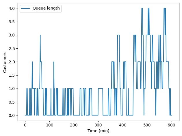
Now we can run the simulation. Here’s a version of run_simulation that creates a TimeSeries with the total number of customers in the store, including the one checking out.

def run_simulation(system, update_func):
    """Simulate a queueing system.
    
    system: System object
    update_func: function object
    """
    x = 0
    results = TimeSeries(name='Queue length')
    results[0] = x
    
    for t in linrange(0, system.duration):
        x = update_func(x, t, system)
        results[t+1] = x

    return results

Call run_simulation with your update function and plot the results.

Hide code cell content
# Solution

results = run_simulation(system, update_func1)
results.plot()
decorate(xlabel='Time (min)', ylabel='Customers')
_images/269ab2747d3af4ce5ce6b2d6fef81dc554cedd4ae9d4c1d9456cc75febdca3b2.png

After the simulation, we can compute L, which is the average number of customers in the system, and W, which is the average time customers spend in the store. L and W are related by Little’s Law:

\(L = \lambda W\)

Where \(\lambda\) is the arrival rate. Here’s a function that computes them.

def compute_metrics(results, system):
    """Compute average number of customers and wait time.
    
    results: TimeSeries of queue lengths
    system: System object
    
    returns: L, W
    """
    L = results.mean()
    W = L / system.lam
    return L, W

Call compute_metrics with the results from your simulation.

Hide code cell content
# Solution

compute_metrics(results, system)
(0.920265780730897, 7.362126245847176)

Parameter sweep#

Since we don’t know the actual value of \(\lambda\), we can sweep through a range of possibilities, from 10% to 80% of the completion rate, \(\mu\). (If customers arrive faster than the completion rate, the queue grows without bound. In that case the metrics L and W just depend on how long the store is open.)

Create an array of values for lam.

Hide code cell content
# Solution

num_vals = 101
lam_array = linspace(0.1*mu, 0.8*mu, num_vals)
lam_array
array([0.02  , 0.0214, 0.0228, 0.0242, 0.0256, 0.027 , 0.0284, 0.0298,
       0.0312, 0.0326, 0.034 , 0.0354, 0.0368, 0.0382, 0.0396, 0.041 ,
       0.0424, 0.0438, 0.0452, 0.0466, 0.048 , 0.0494, 0.0508, 0.0522,
       0.0536, 0.055 , 0.0564, 0.0578, 0.0592, 0.0606, 0.062 , 0.0634,
       0.0648, 0.0662, 0.0676, 0.069 , 0.0704, 0.0718, 0.0732, 0.0746,
       0.076 , 0.0774, 0.0788, 0.0802, 0.0816, 0.083 , 0.0844, 0.0858,
       0.0872, 0.0886, 0.09  , 0.0914, 0.0928, 0.0942, 0.0956, 0.097 ,
       0.0984, 0.0998, 0.1012, 0.1026, 0.104 , 0.1054, 0.1068, 0.1082,
       0.1096, 0.111 , 0.1124, 0.1138, 0.1152, 0.1166, 0.118 , 0.1194,
       0.1208, 0.1222, 0.1236, 0.125 , 0.1264, 0.1278, 0.1292, 0.1306,
       0.132 , 0.1334, 0.1348, 0.1362, 0.1376, 0.139 , 0.1404, 0.1418,
       0.1432, 0.1446, 0.146 , 0.1474, 0.1488, 0.1502, 0.1516, 0.153 ,
       0.1544, 0.1558, 0.1572, 0.1586, 0.16  ])

Write a function that takes an array of values for lam, a single value for mu, and an update function.

For each value of lam, it should run a simulation, compute L and W, and store the value of W in a SweepSeries.

It should return the SweepSeries.

Hide code cell content
# Solution

def sweep_lam(lam_array, mu, update_func):
    """Run simulations with a range of values for `lam`
    
    lam_array: array of values for `lam`
    mu: probability of finishing a checkout
    update_func: passed along to run_simulation
    
    returns: SweepSeries of average wait time vs lam
    """
    sweep = SweepSeries()
    
    for lam in lam_array:
        system = make_system(lam, mu)
        results = run_simulation(system, update_func)
        L, W = compute_metrics(results, system)
        sweep[lam] = W
        
    return sweep

Call your function to generate a SweepSeries, and plot it.

Hide code cell content
# Solution

sweep = sweep_lam(lam_array, mu, update_func1)
Hide code cell content
# Solution

sweep.plot(style='o', alpha=0.5, label='simulation')

decorate(xlabel='Arrival rate, lambda (per min)',
         ylabel='Average time in system',
         title='Single server, single queue')
_images/40666b7afc7e1a3d0c509b0692efa2f0d0af99631bed59aaabacf0bc15c21be0.png

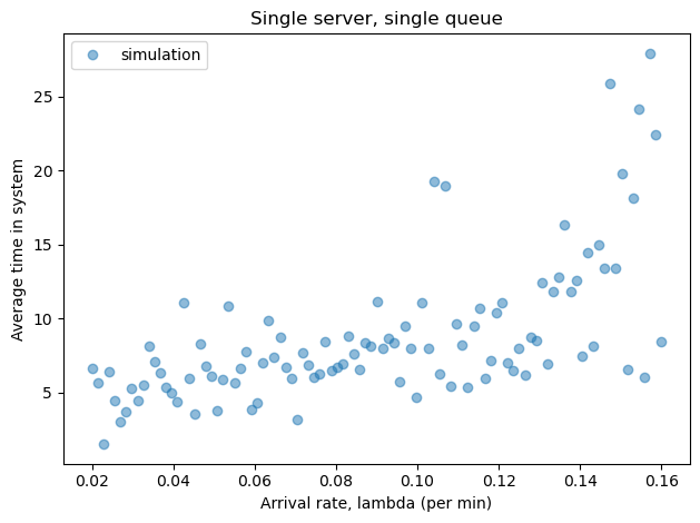
If we imagine that this range of values represents arrival rates on different days, we can use the average value of W, for a range of values of lam, to compare different queueing strategies.
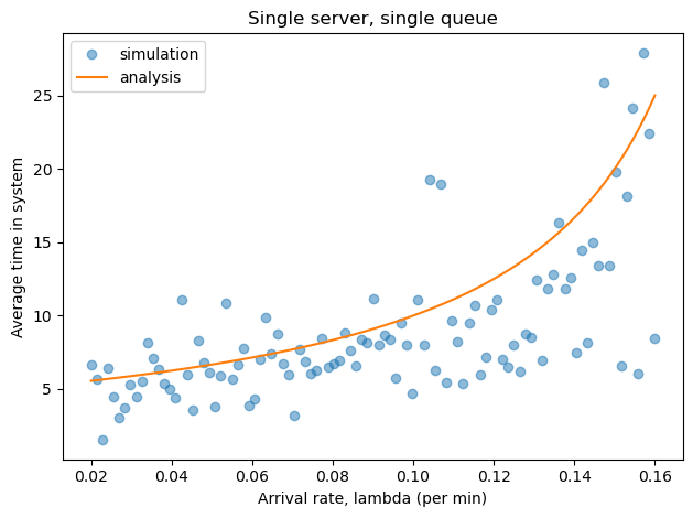
Hide code cell content
# Solution

W_avg = sweep.mean()
W_avg
8.813268411321534

Analysis#

The model I chose for this system is a common model in queueing theory, in part because many of its properties can be derived analytically.

In particular, we can derive the average time in the store as a function of \(\mu\) and \(\lambda\):

\(W = 1 / (\mu - \lambda)\)

The following function plots the theoretical value of \(W\) as a function of \(\lambda\).

def plot_W(lam_array, mu):
    """Plot the theoretical mean wait time.
    
    lam_array: array of values for `lam`
    mu: probability of finishing a checkout
    """
    W_array = 1 / (mu - lam_array)
    W_series = make_series(lam_array, W_array)
    W_series.plot(style='-', label='analysis')

Use this function to plot the theoretical results, then plot your simulation results again on the same graph. How do they compare?
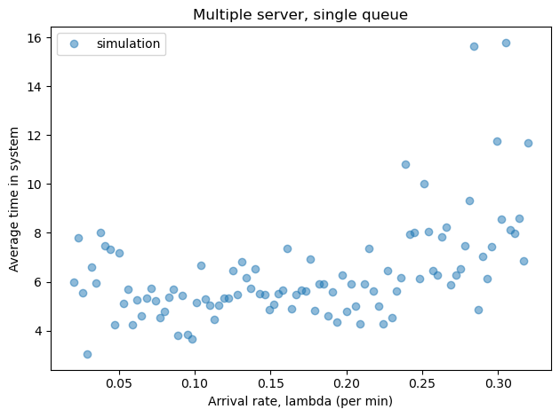
Hide code cell content
# Solution

sweep.plot(style='o', alpha=0.5, label='simulation')
plot_W(lam_array, mu)

decorate(xlabel='Arrival rate, lambda (per min)',
         ylabel='Average time in system',
         title='Single server, single queue')
_images/1e52f320049519d2ec5e67551152b9c99afa8cc5b7579df10cf584d5861b01a1.png

Multiple servers#

Now let’s try the other two queueing strategies:

  1. One queue with two checkout counters.

  2. Two queues, one for each counter.

The following figure shows the three scenarios:

Write an update function for one queue with two servers.

Hide code cell content
# Solution

def update_func2(x, t, system):
    """Simulate a single queue with two servers.
    
    system: System object
    """
    # if both servers are busy, check whether the
    # second is complete
    if x > 1 and flip(system.mu):
        x -= 1
            
    # check whether the first is complete
    if x > 0 and flip(system.mu):
        x -= 1
    
    # check for an arrival
    if flip(system.lam):
        x += 1
        
    return x

Use this update function to simulate the system, plot the results, and print the metrics.

Hide code cell content
# Solution

system = make_system(lam, mu)
run_simulation(system, update_func2)
results.plot()
decorate(xlabel='Time (min)', ylabel='Customers')
compute_metrics(results, system)
(0.920265780730897, 7.362126245847176)
_images/269ab2747d3af4ce5ce6b2d6fef81dc554cedd4ae9d4c1d9456cc75febdca3b2.png

Since we have two checkout counters now, we can consider values for \(\lambda\) that exceed \(\mu\).

Create a new array of values for lam from 10% to 160% of mu.

Hide code cell content
# Solution

lam_array = linspace(0.1*mu, 1.6*mu, num_vals)

Use your sweep function to simulate the two server, one queue scenario with a range of values for lam.

Plot the results and print the average value of W across all values of lam.
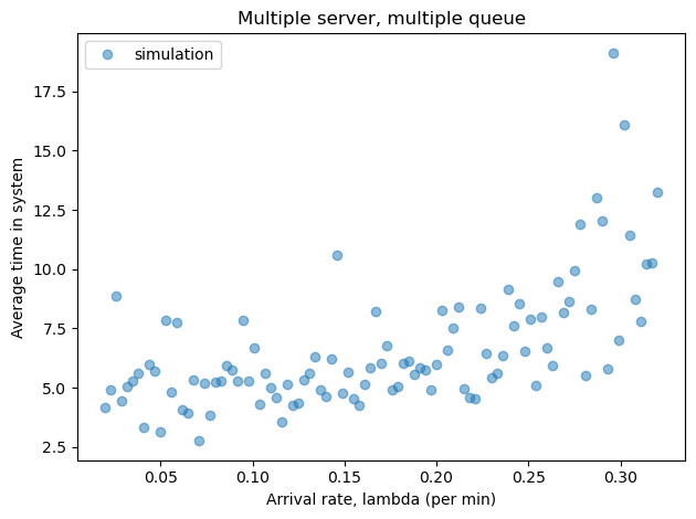
Hide code cell content
# Solution

sweep = sweep_lam(lam_array, mu, update_func2)
W_avg = sweep.mean()
print('Average of averages = ', W_avg, 'minutes')
Average of averages =  6.326606263998706 minutes
Hide code cell content
# Solution

sweep.plot(style='o', alpha=0.5, label='simulation')
decorate(xlabel='Arrival rate, lambda (per min)',
         ylabel='Average time in system',
         title='Multiple server, single queue')
_images/787ddf6f905d304ed39f19b13356685a2e60bc579a17f93d8228ca486be4f438.png

Multiple queues#

To simulate the scenario with two separate queues, we need two state variables to keep track of customers in each queue.

Write an update function that takes x1, x2, t, and system as parameters and returns x1 and x2 as return values. f you are not sure how to return more than one return value, see compute_metrics.

When a customer arrives, which queue do they join?

Hide code cell content
# Solution

def update_func3(x1, x2, t, system):
    """Simulate two queues with one server each.
    
    x1: number of customers in queue 1
    x2: number of customers in queue 2
    t: time step
    system: System object
    """
    # if the first servers is busy, check it it's done
    if x1 > 0 and flip(system.mu):
        x1 -= 1
            
    # if the second queue is busy, check if it's done
    if x2 > 0 and flip(system.mu):
        x2 -= 1
            
    # check for an arrival
    if flip(system.lam):
        # join whichever queue is shorter
        if x1 < x2:
            x1 += 1
        else:
            x2 += 1
            
    return x1, x2

Write a version of run_simulation that works with this update function.

Hide code cell content
# Solution

def run_simulation(system, update_func):
    """Simulate a queueing system.
    
    system: System object
    update_func: function object
    """
    x1, x2 = 0, 0
    results = TimeSeries()
    results[0] = x1 + x2
    
    for t in linrange(0, system.duration):
        x1, x2 = update_func(x1, x2, t, system)
        results[t+1] = x1 + x2

    return results

Test your functions by running a simulation with a single value of lam.

Hide code cell content
# Solution

system = make_system(lam, mu)
run_simulation(system, update_func3)
results.plot()
decorate(xlabel='Time (min)', ylabel='Customers')
compute_metrics(results, system)
(0.920265780730897, 7.362126245847176)
_images/269ab2747d3af4ce5ce6b2d6fef81dc554cedd4ae9d4c1d9456cc75febdca3b2.png

Sweep a range of values for lam, plot the results, and print the average wait time across all values of lam.

How do the results compare to the scenario with two servers and one queue.

Hide code cell content
# Solution

sweep = sweep_lam(lam_array, mu, update_func3)
W_avg = sweep.mean()
print('Average of averages = ', W_avg, 'minutes')
Average of averages =  6.638371020327574 minutes
Hide code cell content
# Solution

sweep.plot(style='o', alpha=0.5, label='simulation')
decorate(xlabel='Arrival rate, lambda (per min)',
         ylabel='Average time in system',
         title='Multiple server, multiple queue')
_images/457853d06e16a58e214628fe04a7739d989fe4e00a72d047c290c29146b75dfb.png
Hide code cell content
# Solution

"""
With two queues, the average of averages is slightly higher, 
most of the time.  But the difference is small.

The two configurations are equally good as long as both servers 
are busy; the only time two lines is worse is if one queue is 
empty and the other contains more than one customer.  
In real life, if we allow customers to change lanes, 
that disadvantage can be eliminated.

From a theoretical point of view, one line is better.  
From a practical point of view, the difference is small 
and can be mitigated.  So the best choice depends on 
practical considerations.

On the other hand, you can do substantially better with 
an express line for customers with short service times.  
But that's a topic for another notebook.
""";

Modeling and Simulation in Python

Copyright 2021 Allen Downey

License: Creative Commons Attribution-NonCommercial-ShareAlike 4.0 International