Drag

Drag#

This chapter is available as a Jupyter notebook where you can read the text, run the code, and work on the exercises. Click here to access the notebooks: https://allendowney.github.io/ModSimPy/.

In the previous chapter we simulated a penny falling in a vacuum, that is, without air resistance. But the computational framework we used is very general; it is easy to add additional forces, including drag.

In this chapter, I present a model of drag force and add it to the simulation.

Drag Force#

As an object moves through a fluid, like air, the object applies force to the air and, in accordance with Newton’s third law of motion, the air applies an equal and opposite force to the object (see http://modsimpy.com/newton).

The direction of this drag force is opposite the direction of travel, and its magnitude is given by the drag equation (see http://modsimpy.com/drageq):

\[F_d = \frac{1}{2}~\rho~v^2~C_d~A\]

where

\(F_d\) is force due to drag, in newtons (N), which are the SI units of force. A newton is 1 kg m/s\(^2\).
\(\rho\) is the density of the fluid in kg/m\(^3\).
\(v\) is the magnitude of velocity in m/s.
\(A\) is the reference area of the object, in m\(^2\). In this context, the reference area is the projected frontal area, that is, the visible area of the object as seen from a point on its line of travel (and far away).
\(C_d\) is the drag coefficient, a dimensionless quantity that depends on the shape of the object (including length but not frontal area), its surface properties, and how it interacts with the fluid.

For objects moving at moderate speeds through air, typical drag coefficients are between 0.1 and 1.0, with blunt objects at the high end of the range and streamlined objects at the low end (see http://modsimpy.com/dragco).

For simple geometric objects we can sometimes guess the drag coefficient with reasonable accuracy; for more complex objects we usually have to take measurements and estimate \(C_d\) from data.

Of course, the drag equation is itself a model, based on the assumption that \(C_d\) does not depend on the other terms in the equation: density, velocity, and area. For objects moving in air at moderate speeds (below 45 mph or 20 m/s), this model might be good enough, but we will revisit this assumption in the next chapter.

For the falling penny, we can use measurements to estimate \(C_d\). In particular, we can measure terminal velocity, \(v_{term}\), which is the speed where drag force equals force due to gravity:

\[\frac{1}{2}~\rho~v_{term}^2~C_d~A = m g\]

where \(m\) is the mass of the object and \(g\) is acceleration due to gravity. Solving this equation for \(C_d\) yields:

\[C_d = \frac{2~m g}{\rho~v_{term}^2~A}\]

According to Mythbusters, the terminal velocity of a penny is between 35 and 65 mph (see http://modsimpy.com/mythbust). Using the low end of their range, 40 mph or about 18 m/s, the estimated value of \(C_d\) is 0.44, which is close to the drag coefficient of a smooth sphere.

Now we are ready to add air resistance to the model. But first I want to introduce one more computational tool, the Params object.

The Params Object#

As the number of system parameters increases, and as we need to do more work to compute them, we will find it useful to define a Params object to contain the quantities we need to make a System object. Params objects are similar to System objects, and we initialize them the same way.

Here’s the Params object for the falling penny:

params = Params(
    mass = 0.0025,      # kg
    diameter = 0.019,   # m
    rho = 1.2,          # kg/m**3
    g = 9.8,            # m/s**2
    v_init = 0,         # m / s
    v_term = 18,        # m / s
    height = 381,       # m
    t_end = 30,         # s
)

The mass and diameter are from http://modsimpy.com/penny. The density of air depends on temperature, barometric pressure (which depends on altitude), humidity, and composition (see http://modsimpy.com/density). I chose a value that might be typical in New York City at 20 °C.

Here’s a version of make_system that takes the Params object and computes the inital state, init, the area, and the coefficient of drag. Then it returns a System object with the quantities we’ll need for the simulation.

from numpy import pi

def make_system(params):
    init = State(y=params.height, v=params.v_init)

    area = pi * (params.diameter/2)**2

    C_d = (2 * params.mass * params.g / 
           (params.rho * area * params.v_term**2))

    return System(init=init,
                  area=area,
                  C_d=C_d,
                  mass=params.mass,
                  rho=params.rho,
                  g=params.g,
                  t_end=params.t_end)

And here’s how we call it.

system = make_system(params)

Based on the mass and diameter of the penny, the density of air, and acceleration due to gravity, and the observed terminal velocity, we estimate that the coefficient of drag is about 0.44.

system.C_d

0.4445009981135434

It might not be obvious why it is useful to create a Params object just to create a System object. In fact, if we run only one simulation, it might not be useful. But it helps when we want to change or sweep the parameters.

For example, suppose we learn that the terminal velocity of a penny is actually closer to 20 m/s. We can make a Params object with the new value, and a corresponding System object, like this:

params2 = params.set(v_term=20)

The result from set is a new Params object that is identical to the original except for the given value of v_term. If we pass params2 to make_system, we see that it computes a different value of C_d.

system2 = make_system(params2)
system2.C_d

0.3600458084719701

If the terminal velocity of the penny is 20 m/s, rather than 18 m/s, that implies that the coefficient of drag is 0.36, rather than 0.44. And that makes sense, since lower drag implies faster terminal velocity.

Using Params objects to make System objects helps make sure that relationships like this are consistent. And since we are always making new objects, rather than modifying existing objects, we are less likely to make a mistake.

Simulating the Penny Drop#

Now let’s get to the simulation. Here’s a version of the slope function that includes drag:

def slope_func(t, state, system):
    y, v = state
    rho, C_d, area = system.rho, system.C_d, system.area
    mass, g = system.mass, system.g
    
    f_drag = rho * v**2 * C_d * area / 2
    a_drag = f_drag / mass
    
    dydt = v
    dvdt = -g + a_drag
    
    return dydt, dvdt

As usual, the parameters of the slope function are a time stamp, a State object, and a System object. We don’t use t in this example, but we can’t leave it out because when run_solve_ivp calls the slope function, it always provides the same arguments, whether they are needed or not.

f_drag is force due to drag, based on the drag equation. a_drag is acceleration due to drag, based on Newton’s second law.

To compute total acceleration, we add accelerations due to gravity and drag. g is negated because it is in the direction of decreasing y; a_drag is positive because it is in the direction of increasing y. In the next chapter we will use Vector objects to keep track of the direction of forces and add them up in a less error-prone way.

As usual, let’s test the slope function with the initial conditions.

slope_func(0, system.init, system)

(0, -9.8)

Because the initial velocity is 0, so is the drag force, so the initial acceleration is still g.

To stop the simulation when the penny hits the sidewalk, we’ll use the event function from the previous chapter.

def event_func(t, state, system):
    y, v = state
    return y

Now we can run the simulation like this:

results, details = run_solve_ivp(system, slope_func,
                                 events=event_func)
details.message

'A termination event occurred.'

Here are the last few time steps:

results.tail()

	y	v
21.541886	1.614743e+01	-18.001510
21.766281	1.211265e+01	-18.006240
21.990676	8.076745e+00	-18.009752
22.215070	4.039275e+00	-18.011553
22.439465	7.105427e-15	-18.011383

The final height is close to 0, as expected.

Interestingly, the final velocity is not exactly terminal velocity, which is a reminder that the simulation results are only approximate.

We can get the flight time from results.

t_sidewalk = results.index[-1]
t_sidewalk

22.43946505804431

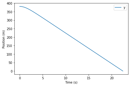
With air resistance, it takes about 22 seconds for the penny to reach the sidewalk.

Here’s a plot of position as a function of time.

def plot_position(results):
    results.y.plot()
        
    decorate(xlabel='Time (s)',
         ylabel='Position (m)')
    
plot_position(results)

_images/ef219430c224573c999bc225f944c7f80f51050bb403f73cab7d9ee75a96dc2b.png

And velocity as a function of time:

def plot_velocity(results):

    results.v.plot(color='C1', label='v')
        
    decorate(xlabel='Time (s)',
             ylabel='Velocity (m/s)')
    
plot_velocity(results)

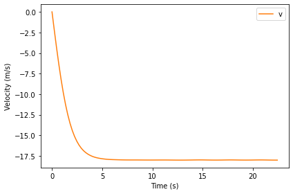
_images/6293c039285bb7a86a8cfa0c9f5923d89167c9d0b6229ad9b608c11a4e428f44.png

From an initial velocity of 0, the penny accelerates downward until it reaches terminal velocity; after that, velocity is constant.

Summary#

This chapter presents a model of drag force, which we use to estimate the coefficient of drag for a penny, and then simulate, one more time, dropping a penny from the Empire State Building.

In the next chapter we’ll move from one dimension to two, simulating the flight of a baseball. But first you might want to work on these exercises.

Exercises#

This chapter is available as a Jupyter notebook where you can read the text, run the code, and work on the exercises. You can access the notebooks at https://allendowney.github.io/ModSimPy/.

Exercise 1#

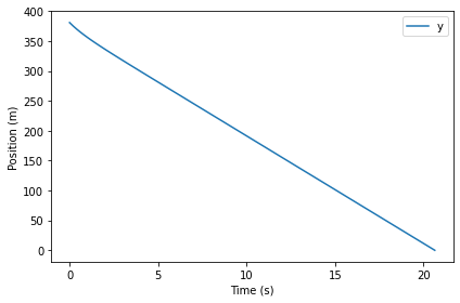
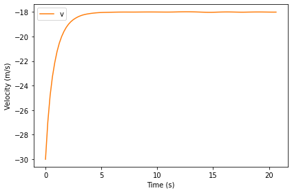
Run the simulation with a downward initial velocity that exceeds the penny’s terminal velocity.

What do you expect to happen? Plot velocity and position as a function of time, and see if they are consistent with your prediction.

Hint: Use params.set to make a new Params object with a different initial velocity.

Exercise 2#

Suppose we drop a quarter from the Empire State Building and find that its flight time is 19.1 seconds. Use this measurement to estimate terminal velocity and coefficient of drag.

You can get the relevant dimensions of a quarter from https://en.wikipedia.org/wiki/Quarter_(United_States_coin).

Create a Params object with new values of mass and diameter. We don’t know v_term, so we’ll start with the initial guess 18 m/s.
Use make_system to create a System object.
Call run_solve_ivp to simulate the system. How does the flight time of the simulation compare to the measurement?
Try a few different values of v_term and see if you can get the simulated flight time close to 19.1 seconds.
Optionally, write an error function and use root_scalar to improve your estimate.
Use your best estimate of v_term to compute C_d.

Note: I fabricated the “observed” flight time, so don’t take the results of this exercise too seriously.