Case Studies Part 1

Case Studies Part 1#

This chapter presents case studies where you can apply the tools we have learned so far to problems involving population growth, queueing systems, and tree growth.

This chapter is available as a Jupyter notebook where you can read the text, run the code, and work on the exercises. Click here to access the notebooks: https://allendowney.github.io/ModSimPy/.

Historical World Population#

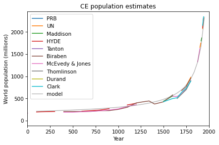
The Wikipedia page about world population growth includes estimates for world population from 12,000 years ago to the present (see https://en.wikipedia.org/wiki/World_population_estimates.html).

The following figure shows the estimates of several research groups from 1 CE to the near present.

table1.plot()
decorate(xlim=[0, 2000], xlabel='Year', 
         ylabel='World population (millions)',
         title='CE population estimates')

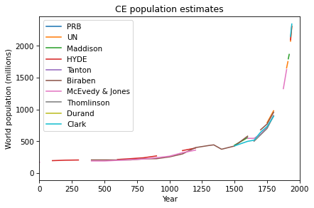
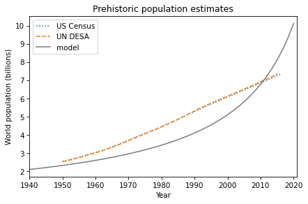
_images/3e2d6728c647783e46c895cdec7b80a1f5b60b6c3f3c82d7a0e2ae16801842e7.png

See if you can find a model that fits these estimates. How well does your best model predict actual population growth from 1940 to the present?

One Queue Or Two?#

This case study is related to queueing theory, which is the study of systems that involve waiting in lines, also known as “queues”.

Suppose you are designing the checkout area for a new store. There is enough room in the store for two checkout counters and a waiting area for customers. You can make two lines, one for each counter, or one line that feeds both counters.

In theory, you might expect a single line to be better, but it has some practical drawbacks: in order to maintain a single line, you might have to install barriers, and customers might be put off by what seems to be a longer line, even if it moves faster.

So you’d like to check whether the single line is really better and by how much. Simulation can help answer this question.

This figure shows the three scenarios we’ll consider:

One queue, one server (left), one queue, two servers (middle), two queues, two servers (right).

As we did in the bike share model, we’ll divide time into discrete time steps of one minute. And we’ll assume that a customer is equally likely to arrive during any time step. I’ll denote this probability using the Greek letter lambda, \(\lambda\), or the variable name lam. The value of \(\lambda\) probably varies from day to day, so we’ll have to consider a range of possibilities.

Based on data from other stores, you know that it takes 5 minutes for a customer to check out, on average. But checkout times are variable: most customers take less than 5 minutes, but some take substantially more. A simple way to model this variability is to assume that when a customer is checking out, they always have the same probability of finishing during the next time step, regardless of how long they have been checking out. I’ll denote this probability using the Greek letter mu, \(\mu\), or the variable name mu.

If we choose \(\mu=1/5\) per minute, the average time for each checkout will be 5 minutes, which is consistent with the data. Most people take less than 5 minutes, but a few take substantially longer, which is probably not a bad model of the distribution in real stores.

Now we’re ready to implement the model. In the repository for this book, you’ll find a notebook called queue.ipynb that contains some code to get you started and instructions. You can download it from AllenDowney/ModSimPy or run it on Colab at https://colab.research.google.com/github/AllenDowney/ModSimPy/blob/master/examples/queue.ipynb.

As always, you should practice incremental development: write no more than one or two lines of code at a time, and test as you go!

Predicting Salmon Populations#

Each year the U.S. Atlantic Salmon Assessment Committee reports estimates of salmon populations in oceans and rivers in the northeastern United States. The reports are useful for monitoring changes in these populations, but they generally do not include predictions.

The goal of this case study is to model year-to-year changes in population, evaluate how predictable these changes are, and estimate the probability that a particular population will increase or decrease in the next 10 years.

As an example, I use data from the 2017 report, which provides population estimates for the Narraguagus and Sheepscot Rivers in Maine.

In the repository for this book, you’ll find a notebook called salmon.ipynb that contains this data and some code to get you started. You can download it from AllenDowney/ModSimPy or run it on Colab at https://colab.research.google.com/github/AllenDowney/ModSimPy/blob/master/examples/salmon.ipynb.

You should take my instructions as suggestions; if you want to try something different, please do!

Tree Growth#

This case study is based on “Height-Age Curves for Planted Stands of Douglas Fir, with Adjustments for Density”, a working paper by Flewelling et al. It provides site index curves, which are curves that show the expected height of the tallest tree in a stand of Douglas fir as a function of age, for a stand where the trees are the same age. Depending on the quality of the site, the trees might grow more quickly or slowly. So each curve is identified by a site index that indicates the quality of the site.

The goal of this case study is to explain the shape of these curves, that is, why trees grow the way they do. The answer I propose involves fractal dimensions, so you might find it interesting.

In the repository for this book, you’ll find a notebook called trees.ipynb that incrementally develops a model of tree growth and uses it to fit the data. You can download it from AllenDowney/ModSimPy or run it on Colab at https://colab.research.google.com/github/AllenDowney/ModSimPy/blob/master/examples/trees.ipynb.

There are no exercises in this case study, but it is an example of what you can do with the tools we have so far and a preview of what you will be able to do with the tools in the next few chapters.