Printed and electronic copies of Modeling and Simulation in Python are available from No Starch Press and Bookshop.org and Amazon.
Sweeping Parameters#
In the previous chapter we extended the Kermack-McKendrick (KM) model to include immunization and used it to demonstrate herd immunity.
But we assumed that the parameters of the model, contact rate and recovery rate, were known. In this chapter, we’ll explore the behavior of the model as we vary these parameters.
In the next chapter, we’ll use analysis to understand these relationships better, and propose a method for using data to estimate parameters.
Sweeping Beta#
Recall that \(\beta\) is the contact rate, which captures both the frequency of interaction between people and the fraction of those interactions that result in a new infection. If \(N\) is the size of the population and \(s\) is the fraction that’s susceptible, \(s N\) is the number of susceptibles, \(\beta s N\) is the number of contacts per day between susceptibles and other people, and \(\beta s i N\) is the number of those contacts where the other person is infectious.
As \(\beta\) increases, we expect the total number of infections to increase. To quantify that relationship, I’ll create a range of values for \(\beta\):
beta_array = linspace(0.1, 1.1, 11)
gamma = 0.25
We’ll start with a single value for gamma, which is the recovery rate, that is, the fraction of infected people who recover per day.
The following function takes beta_array and gamma as parameters.
It runs the simulation for each value of beta and computes the same metric we used in the previous chapter, the fraction of the population that gets infected.
The result is a SweepSeries that contains the values of beta and the corresponding metrics.
def sweep_beta(beta_array, gamma):
    sweep = SweepSeries()
    for beta in beta_array:
        system = make_system(beta, gamma)
        results = run_simulation(system, update_func)
        sweep[beta] = calc_total_infected(results, system)
    return sweep
We can run sweep_beta like this:
infected_sweep = sweep_beta(beta_array, gamma)
Before we plot the results, I will use a formatted string literal, also called an f-string to assemble a label that includes the value of gamma:
label = f'gamma = {gamma}'
label
'gamma = 0.25'
An f-string starts with the letter f followed by a string in single or double quotes.
The string can contain any number of format specifiers in squiggly brackets, {}.
When a variable name appears in a format specifier, it is replaced with the value of the variable.
In this example, the value of gamma is 0.25, so the value of label is 'gamma = 0.25'.
You can read more about f-strings at https://docs.python.org/3/tutorial/inputoutput.html#tut-f-strings.
Now let’s see the results.
infected_sweep.plot(label=label, color='C1')

decorate(xlabel='Contact rate (beta)',
         ylabel='Fraction infected')
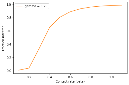
Remember that this figure
is a parameter sweep, not a time series, so the x-axis is the parameter
beta, not time.
When beta is small, the contact rate is low and the outbreak never
really takes off; the total number of infected students is near zero. As
beta increases, it reaches a threshold near 0.3 where the fraction of
infected students increases quickly. When beta exceeds 0.5, more than
80% of the population gets sick.
Sweeping Gamma#
Let’s see what that looks like for a few different values of gamma.
We’ll use linspace to make an array of values:
gamma_array = linspace(0.1, 0.7, 4)
gamma_array
array([0.1, 0.3, 0.5, 0.7])
And run sweep_beta for each value of gamma:
for gamma in gamma_array:
    infected_sweep = sweep_beta(beta_array, gamma)
    label = f'gamma = {gamma}'
    infected_sweep.plot(label=label)

decorate(xlabel='Contact rate (beta)',
         ylabel='Fraction infected')
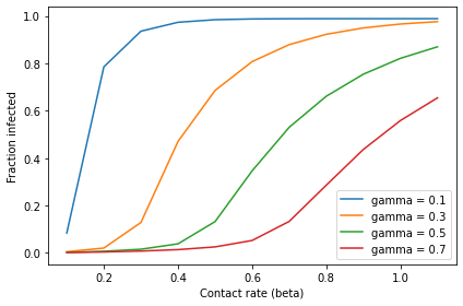
When gamma is low, the recovery rate is low, which means people are infectious longer.
In that case, even a low contact rate (beta) results in an epidemic.
When gamma is high, beta has to be even higher to get things going.
Using a SweepFrame#
In the previous section, we swept a range of values for gamma, and for
each value of gamma, we swept a range of values for beta. This process is a
two-dimensional sweep.
If we want to store the results, rather than plot them, we can use a
SweepFrame, which is a kind of DataFrame where the rows sweep one
parameter, the columns sweep another parameter, and the values contain
metrics from a simulation.
This function shows how it works:
def sweep_parameters(beta_array, gamma_array):
    frame = SweepFrame(columns=gamma_array)
    for gamma in gamma_array:
        frame[gamma] = sweep_beta(beta_array, gamma)
    return frame
sweep_parameters takes as parameters an array of values for beta and
an array of values for gamma.
It creates a SweepFrame to store the results, with one column for each
value of gamma and one row for each value of beta.
Each time through the loop, we run sweep_beta. The result is a
SweepSeries object with one element for each value of beta. The
assignment inside the loop stores the SweepSeries as a new column in
the SweepFrame, corresponding to the current value of gamma.
At the end, the SweepFrame stores the fraction of students infected
for each pair of parameters, beta and gamma.
We can run sweep_parameters like this:
frame = sweep_parameters(beta_array, gamma_array)
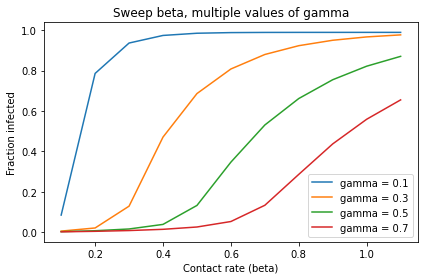
With the results in a SweepFrame, we can plot each column like this:
for gamma in gamma_array:
    label = f'gamma = {gamma}'
    frame[gamma].plot(label=label)

decorate(xlabel='Contact rate (beta)',
         ylabel='Fraction infected',
         title='Sweep beta, multiple values of gamma')
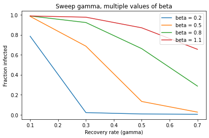
Alternatively, we can plot each row like this:
for beta in [0.2, 0.5, 0.8, 1.1]:
    label = f'beta = {beta}'
    frame.loc[beta].plot(label=label)

decorate(xlabel='Recovery rate (gamma)',
         ylabel='Fraction infected',
         title='Sweep gamma, multiple values of beta')
This example demonstrates one use of a SweepFrame: we can run the analysis once, save the results, and then generate different visualizations.
Another way to visualize the results of a two-dimensional sweep is a contour plot, which shows the parameters on the axes and contour lines where the value of the metric is constant.
The ModSim library provides contour, which takes a SweepFrame and uses Matplotlib to generate a contour plot.
contour(frame)

decorate(xlabel='Recovery rate (gamma)',
         ylabel='Contact rate (beta)',
         title='Contour plot, fraction infected')
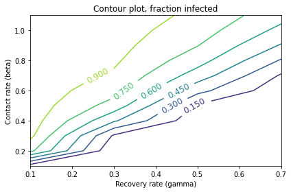
The values of gamma are on the \(x\)-axis, corresponding to the columns of the SweepFrame.
The values of beta are on the \(y\)-axis, corresponding to the rows of the SweepFrame.
Each line follows a contour where the infection rate is constant.
Infection rates are lowest in the lower right, where the contact rate is low and the recovery rate is high. They increase as we move to the upper left, where the contact rate is high and the recovery rate is low.
Summary#
This chapter demonstrates a two-dimensional parameter sweep using a SweepFrame to store the results.
We plotted the results three ways:
First we plotted total infections versus
beta, with one line for each value ofgamma.Then we plotted total infections versus
gamma, with one line for each value ofbeta.Finally, we made a contour plot with
betaon the \(y\)-axis,gammaon the \(x\)-axis and contour lines where the metric is constant.
These visualizations suggest that there is a relationship between beta and gamma that determines the outcome of the model.
In fact, there is.
In the next chapter we’ll explore it by running simulations, then derive it by analysis.
Exercises#
This chapter is available as a Jupyter notebook where you can read the text, run the code, and work on the exercises. You can access the notebooks at https://allendowney.github.io/ModSimPy/.
Exercise 1#
If we know beta and gamma, we can compute the fraction of the population that gets infected. In general, we don’t know these parameters, but sometimes we can estimate them based on the behavior of an outbreak.
Suppose the infectious period for the Freshman Plague is known to be 2 days on average, and suppose during one particularly bad year, 40% of the class is infected at some point. Estimate the time between contacts, 1/beta.