Sweeping Parameters

Sweeping Parameters#

In the previous chapter we defined metrics that quantify the performance of a bike sharing system. In this chapter we’ll see how those metrics depend on the parameters of the system, like the arrival rate of customers at the stations.

And I will present a program development strategy, called incremental development, that might help you write programs faster and spend less time debugging.

This chapter is available as a Jupyter notebook where you can read the text, run the code, and work on the exercises. Click here to access the notebooks: https://allendowney.github.io/ModSimPy/.

Functions That Return Values#

We have used several functions that return values. For example, when you run sqrt, it returns a number you can assign to a variable.

from numpy import sqrt

root_2 = sqrt(2)
root_2

1.4142135623730951

And when you run State, it returns a new State object:

bikeshare = State(olin=10, wellesley=2)
bikeshare

olin         10
wellesley     2
Name: state, dtype: int64

Not all functions have return values. For example, when you run step, it updates a State object, but it doesn’t return a value.

To write functions that return values, we can use a return statement, like this:

def add_five(x):
    return x + 5

add_five takes a parameter, x, which could be any number. It computes x + 5 and returns the result. So if we run it like this, the result is 8:

add_five(3)

As a more useful example, here’s a version of run_simulation that creates a State object, runs a simulation, and then returns the State object:

def run_simulation(p1, p2, num_steps):
    state = State(olin=10, wellesley=2,
                  olin_empty=0, wellesley_empty=0)
    
    for i in range(num_steps):
        step(state, p1, p2)
        
    return state

We can call run_simulation like this:

final_state = run_simulation(0.3, 0.2, 60)

The result is a State object that represents the final state of the system, including the metrics we’ll use to evaluate the performance of the system:

print(final_state.olin_empty, 
      final_state.wellesley_empty)

0 0

The simulation we just ran starts with olin=10 and wellesley=2, and uses the values p1=0.3, p2=0.2, and num_steps=60. These five values are parameters of the model, which are quantities that determine the behavior of the system.

It is easy to get the parameters of a model confused with the parameters of a function. It is especially easy because the parameters of a model often appear as parameters of a function.

For example, the previous version of run_simulation takes p1, p2, and num_steps as parameters. So we can call run_simulation with different parameters and see how the metrics, like the number of unhappy customers, depend on the parameters. But before we do that, we need a new version of a for loop.

Loops and Arrays#

In run_simulation, we use this for loop:

    for i in range(num_steps):
        step(state, p1, p2)

In this example, range creates a sequence of numbers from 0 to num_steps (including 0 but not num_steps). Each time through the loop, the next number in the sequence gets assigned to the loop variable, i.

But range only works with integers; to get a sequence of non-integer values, we can use linspace, which is provided by NumPy:

from numpy import linspace

p1_array = linspace(0, 1, 5)
p1_array

array([0.  , 0.25, 0.5 , 0.75, 1.  ])

The arguments indicate where the sequence should start and stop, and how many elements it should contain. In this example, the sequence contains 5 equally-spaced numbers, starting at 0 and ending at 1.

The result is a NumPy array, which is a new kind of object we have not seen before. An array is a container for a sequence of numbers.

We can use an array in a for loop like this:

for p1 in p1_array:
    print(p1)

When this loop runs, it

Gets the first value from the array and assigns it to p1.
Runs the body of the loop, which prints p1.
Gets the next value from the array and assigns it to p1.
Runs the body of the loop, which prints p1.
…

And so on, until it gets to the end of the array. This will come in handy in the next section.

Sweeping Parameters#

If we know the actual values of parameters like p1 and p2, we can use them to make specific predictions, like how many bikes will be at Olin after one hour.

But prediction is not the only goal; models like this are also used to explain why systems behave as they do and to evaluate alternative designs. For example, if we observe the system and notice that we often run out of bikes at a particular time, we could use the model to figure out why that happens. And if we are considering adding more bikes, or another station, we could evaluate the effect of various “what if” scenarios.

As an example, suppose we have enough data to estimate that p2 is about 0.2, but we don’t have any information about p1. We could run simulations with a range of values for p1 and see how the results vary. This process is called sweeping a parameter, in the sense that the value of the parameter “sweeps” through a range of possible values.

Now that we know about loops and arrays, we can use them like this:

p1_array = linspace(0, 0.6, 6)
p2 = 0.2
num_steps = 60

for p1 in p1_array:
    final_state = run_simulation(p1, p2, num_steps)
    print(p1, final_state.olin_empty)

Each time through the loop, we run a simulation with a different value of p1 and the same value of p2, 0.2. Then we print p1 and the number of unhappy customers at Olin.

To save and plot the results, we can use a SweepSeries object, which is similar to a TimeSeries; the difference is that the labels in a SweepSeries are parameter values rather than time values.

We can create an empty SweepSeries like this:

sweep = SweepSeries()

And add values like this:

p1_array = linspace(0, 0.6, 31)

for p1 in p1_array:
    final_state = run_simulation(p1, p2, num_steps)
    sweep[p1] = final_state.olin_empty

The result is a SweepSeries that maps from each value of p1 to the resulting number of unhappy customers.

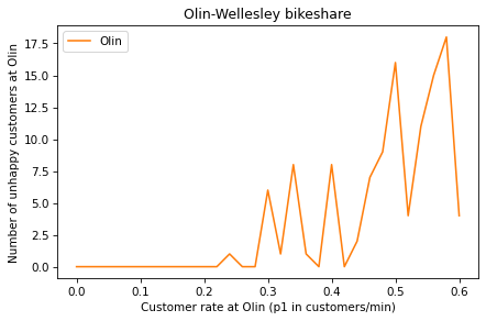
We can plot the elements of the SweepSeries like this:

sweep.plot(label='Olin', color='C1')

decorate(title='Olin-Wellesley bikeshare',
         xlabel='Customer rate at Olin (p1 in customers/min)', 
         ylabel='Number of unhappy customers at Olin')

_images/5a8e4eda21b18c20426408da9e6c8e973b9ee9d6e9ae229b6cb8b1fb01b3ecb8.png

The keyword argument color='C1' specifies the color of the line. The TimeSeries we have plotted so far use the default color, C0, which is blue (see https://matplotlib.org/stable/tutorials/colors/colors.html for the other colors defined by Matplotlib). I use a different color for SweepSeries to remind us that it is not a TimeSeries.

When the arrival rate at Olin is low, there are plenty of bikes and no unhappy customers. As the arrival rate increases, we are more likely to run out of bikes and the number of unhappy customers increases. The line is jagged because the simulation is based on random numbers. Sometimes we get lucky and there are relatively few unhappy customers; other times we are unlucky and there are more.

Incremental Development#

When you start writing programs that are more than a few lines, you might find yourself spending more time debugging. The more code you write before you start debugging, the harder it is to find the problem.

Incremental development is a way of programming that tries to minimize the pain of debugging. The fundamental steps are:

Always start with a working program. If you have an example from a book, or a program you wrote that is similar to what you are working on, start with that. Otherwise, start with something you know is correct, like x=5. Run the program and confirm that it does what you expect.
Make one small, testable change at a time. A “testable” change is one that displays something or has some other effect you can check. Ideally, you should know what the correct answer is, or be able to check it by performing another computation.
Run the program and see if the change worked. If so, go back to Step 2. If not, you have to do some debugging, but if the change you made was small, it shouldn’t take long to find the problem.

When this process works, your changes usually work the first time or, if they don’t, the problem is obvious. In practice, there are two problems with incremental development:

Sometimes you have to write extra code to generate visible output that you can check. This extra code is called scaffolding because you use it to build the program and then remove it when you are done. That might seem like a waste, but time you spend on scaffolding is almost always time you save on debugging.
When you are getting started, it might not be obvious how to choose the steps that get from x=5 to the program you are trying to write. You will see more examples of this process as we go along, and you will get better with experience.

If you find yourself writing more than a few lines of code before you start testing, and you are spending a lot of time debugging, try incremental development.

Summary#

This chapter introduces functions that return values, which we use to write a version of run_simulation that returns a State object with the final state of the system.

It also introduces linspace, which we use to create a NumPy array, and SweepSeries, which we use to store the results of a parameter sweep.

We used a parameter sweep to explore the relationship between one of the parameters, p1, and the number of unhappy customers, which is a metric that quantifies how well (or badly) the system works.

In the exercises, you’ll have a chance to sweep other parameters and compute other metrics.

In the next chapter, we’ll move on to a new problem, modeling and predicting world population growth.

Exercises#

Exercise 1#

Write a function called make_state that creates a State object with the state variables olin=10 and wellesley=2, and then returns the new State object.

Write a line of code that calls make_state and assigns the result to a variable named init.

Show code cell content Hide code cell content

# Solution

init = make_state()
show(init)

	state
olin	10
wellesley	2

Exercise 2#

Read the documentation of linspace at https://numpy.org/doc/stable/reference/generated/numpy.linspace.html. Then use it to make an array of 101 equally spaced points between 0 and 1 (including both).

Exercise 3#

Wrap the code from this chapter in a function named sweep_p1 that takes an array called p1_array as a parameter. It should create a new SweepSeries and run a simulation for each value of p1 in p1_array, with p2=0.2 and num_steps=60. It should store the results in the SweepSeries and return it.

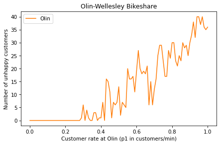
Use your function to generate a SweepSeries and then plot the number of unhappy customers at Olin as a function of p1. Label the axes.

Exercise 4#

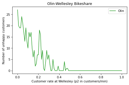
Write a function called sweep_p2 that runs simulations with p1=0.5 and a range of values for p2. It should store the results in a SweepSeries and return the SweepSeries.

Challenge Exercises#

The following two exercises are a little more challenging. If you are comfortable with what you have learned so far, you should give them a try. If you feel like you have your hands full, you might want to skip them for now.

Exercise 5#

Because our simulations are random, the results vary from one run to another, and the results of a parameter sweep tend to be noisy. We can get a clearer picture of the relationship between a parameter and a metric by running multiple simulations with the same parameter and taking the average of the results.

Write a function called run_multiple_simulations that takes as parameters p1, p2, num_steps, and num_runs. num_runs specifies how many times it should call run_simulation.

After each run, it should store the total number of unhappy customers (at Olin or Wellesley) in a TimeSeries. At the end, it should return the TimeSeries.

Test your function with parameters

p1 = 0.3
p2 = 0.3
num_steps = 60
num_runs = 10

Display the resulting TimeSeries and use the mean function from NumPy to compute the average number of unhappy customers.

Show code cell content Hide code cell content

# Solution

p1 = 0.3
p2 = 0.3
num_steps = 60
num_runs = 10
totals = run_multiple_simulations(p1, p2, num_steps, num_runs)
show(totals)

	Quantity
Time
0	0
1	3
2	0
3	0
4	5
5	5
6	0
7	4
8	2
9	0

Exercise 6#

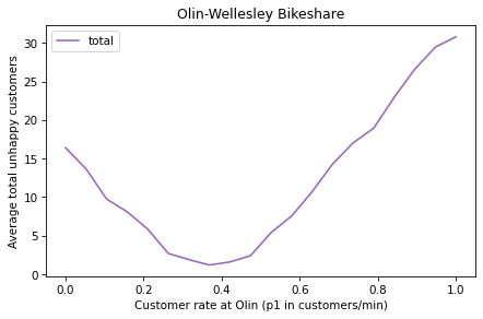
Continuing the previous exercise, use run_multiple_simulations to run simulations with a range of values for p1 and p2.

p2 = 0.3
num_steps = 60
num_runs = 20

Store the results in a SweepSeries, then plot the average number of unhappy customers as a function of p1. Label the axes.

What value of p1 minimizes the average number of unhappy customers?

Under the Hood#

The object you get when you call SweepSeries is actually a Pandas Series, the same as the object you get from TimeSeries. I give them different names to help us remember that they play different roles.

Series provides a number of functions, which you can read about at https://pandas.pydata.org/pandas-docs/stable/reference/api/pandas.Series.html.

They include mean, which computes the average of the values in the Series, so if you have a Series named totals, for example, you can compute the mean like this:

    totals.mean()

Series provides other statistical functions, like std, which computes the standard deviation of the values in the series.

In this chapter I use the keyword argument color to specify the color of a line plot. You can read about the other available colors at https://matplotlib.org/3.3.2/tutorials/colors/colors.html.

Sweeping Parameters

Contents

Sweeping Parameters#

Functions That Return Values#

Loops and Arrays#

Sweeping Parameters#

Incremental Development#

Summary#

Exercises#

Exercise 1#

Exercise 2#

Exercise 3#

Exercise 4#

Challenge Exercises#

Exercise 5#

Exercise 6#

Under the Hood#