The Empire State Building Strikes Back

The Empire State Building Strikes Back#

This chapter is available as a Jupyter notebook where you can read the text, run the code, and work on the exercises. Click here to access the notebooks: https://allendowney.github.io/ModSimPy/.

So far the differential equations we’ve worked with have been first order, which means they involve only first derivatives. In this chapter, we turn our attention to second order differential equations, which can involve both first and second derivatives.

We’ll revisit the falling penny example from Chapter 1, and use run_solve_ivp to find the position and velocity of the penny as it falls, with and without air resistance.

Newton’s Second Law of Motion#

First order differential equations (DEs) can be written

\[\frac{dy}{dx} = G(x, y)\]

where \(G\) is some function of \(x\) and \(y\) (see http://modsimpy.com/ode). Second order DEs can be written

\[\frac{d^2y}{dx^2} = H(x, y, \frac{dy}{dt})\]

where \(H\) is a function of \(x\), \(y\), and \(dy/dx\).

In this chapter, we will work with one of the most famous and useful second order DEs, Newton’s second law of motion:

\[F = m a\]

where \(F\) is a force or the total of a set of forces, \(m\) is the mass of a moving object, and \(a\) is its acceleration.

Newton’s law might not look like a differential equation, until we realize that acceleration, \(a\), is the second derivative of position, \(y\), with respect to time, \(t\). With the substitution

\[a = \frac{d^2y}{dt^2}\]

Newton’s law can be written

\[\frac{d^2y}{dt^2} = F / m\]

And that’s definitely a second order DE. In general, \(F\) can be a function of time, position, and velocity.

Of course, this “law” is really a model in the sense that it is a simplification of the real world. Although it is often approximately true:

It only applies if \(m\) is constant. If mass depends on time, position, or velocity, we have to use a more general form of Newton’s law (see http://modsimpy.com/varmass).
It is not a good model for very small things, which are better described by another model, quantum mechanics.
And it is not a good model for things moving very fast, which are better described by yet another model, relativistic mechanics.

However, for medium-sized things with constant mass, moving at medium-sized speeds, Newton’s model is extremely useful. If we can quantify the forces that act on such an object, we can predict how it will move.

Dropping Pennies#

As a first example, let’s get back to the penny falling from the Empire State Building, which we considered in Chapter 1. We will implement two models of this system: first without air resistance, then with.

Given that the Empire State Building is 381 m high, and assuming that the penny is dropped from a standstill, the initial conditions are:

init = State(y=381, v=0)

where y is height above the sidewalk and v is velocity.

I’ll put the initial conditions in a System object, along with the magnitude of acceleration due to gravity, g, and the duration of the simulations, t_end.

system = System(init=init, 
                g=9.8, 
                t_end=10)

Now we need a slope function, and here’s where things get tricky. As we have seen, run_solve_ivp can solve systems of first order DEs, but Newton’s law is a second order DE. However, if we recognize that

Velocity, \(v\), is the derivative of position, \(dy/dt\), and
Acceleration, \(a\), is the derivative of velocity, \(dv/dt\),

we can rewrite Newton’s law as a system of first order ODEs:

\[\frac{dy}{dt} = v\]

\[\frac{dv}{dt} = a\]

And we can translate those equations into a slope function:

def slope_func(t, state, system):
    y, v = state

    dydt = v
    dvdt = -system.g
    
    return dydt, dvdt

As usual, the parameters are a time stamp, a State object, and a System object.

The first line unpacks the state variables, y and v.

The next two lines compute the derivatives of the state variables, dydt and dvdt. The derivative of position is velocity, and the derivative of velocity is acceleration. In this case, \(a = -g\), which indicates that acceleration due to gravity is in the direction of decreasing \(y\).

slope_func returns a sequence containing the two derivatives.

Before calling run_solve_ivp, it is a good idea to test the slope function with the initial conditions:

dydt, dvdt = slope_func(0, system.init, system)
dydt, dvdt

(0, -9.8)

The result is 0 m/s for velocity and -9.8 m/s\(^2\) for acceleration.

Now we call run_solve_ivp like this:

results, details = run_solve_ivp(system, slope_func)
details.message

'The solver successfully reached the end of the integration interval.'

results is a TimeFrame with two columns: y contains the height of the penny; v contains its velocity. Here are the first few rows.

results.head()

	y	v
0.0	381.000	0.00
0.1	380.951	-0.98
0.2	380.804	-1.96
0.3	380.559	-2.94
0.4	380.216	-3.92

We can plot the results like this:

results.y.plot()

decorate(xlabel='Time (s)',
         ylabel='Position (m)')

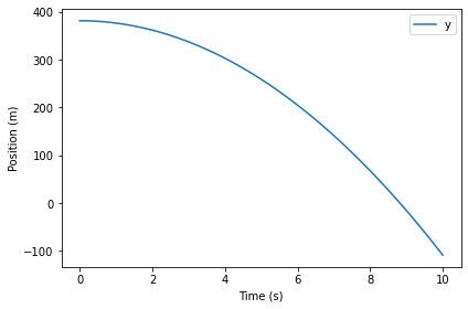
_images/36ec1cc4dce59081de959bcc799da15cb722b0fafdb0af3895ff99b962b1dc15.png

Since acceleration is constant, velocity increases linearly and position decreases quadratically; as a result, the height curve is a parabola.

The last value of results.y is negative, which means we ran the simulation too long.

results.iloc[-1].y

-108.99999999999869

One way to solve this problem is to use the results to estimate the time when the penny hits the sidewalk.

The ModSim library provides crossings, which takes a TimeSeries and a value, and returns a sequence of times when the series passes through the value. We can find the time when the height of the penny is 0 like this:

t_crossings = crossings(results.y, 0)
t_crossings

array([8.81788535])

The result is an array with a single value, 8.818 s. Now, we could run the simulation again with t_end = 8.818, but there’s a better way.

Events#

As an option, run_solve_ivp can take an event function, which detects an “event”, like the penny hitting the sidewalk, and ends the simulation.

Event functions take the same parameters as slope functions, t, state, and system. They should return a value that passes through 0 when the event occurs. Here’s an event function that detects the penny hitting the sidewalk:

def event_func(t, state, system):
    y, v = state
    return y

The return value is the height of the penny, y, which passes through 0 when the penny hits the sidewalk.

We pass the event function to run_solve_ivp like this:

results, details = run_solve_ivp(system, slope_func,
                                 events=event_func)
details.message

'A termination event occurred.'

Then we can get the flight time like this:

t_end = results.index[-1]
t_end

8.81788534972056

And the final velocity like this:

y, v = results.iloc[-1]
y, v

(5.684341886080802e-14, -86.4152764272615)

If there were no air resistance, the penny would hit the sidewalk (or someone’s head) at about 86 m/s. So it’s a good thing there is air resistance.

Summary#

In this chapter, we wrote Newton’s second law, which is a second order DE, as a system of first order DEs. Then we used run_solve_ivp to simulate a penny dropping from the Empire State Building in the absence of air resistance. And we used an event function to stop the simulation when the penny reaches the sidewalk.

In the next chapter we’ll add air resistance to the model. But first you might want to work on this exercise.

Exercises#

This chapter is available as a Jupyter notebook where you can read the text, run the code, and work on the exercises. You can access the notebooks at https://allendowney.github.io/ModSimPy/.

Exercise 1#

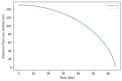
Here’s a question from the web site Ask an Astronomer (see http://curious.astro.cornell.edu/about-us/39-our-solar-system/the-earth/other-catastrophes/57-how-long-would-it-take-the-earth-to-fall-into-the-sun-intermediate):

“If the Earth suddenly stopped orbiting the Sun, I know eventually it would be pulled in by the Sun’s gravity and hit it. How long would it take the Earth to hit the Sun? I imagine it would go slowly at first and then pick up speed.”

Use run_solve_ivp to answer this question.

Here are some suggestions about how to proceed:

Look up the Law of Universal Gravitation and any constants you need. I suggest you work entirely in SI units: meters, kilograms, and Newtons.
When the distance between the Earth and the Sun gets small, this system behaves badly, so you should use an event function to stop when the surface of Earth reaches the surface of the Sun.
Express your answer in days, and plot the results as millions of kilometers versus days.

If you read the reply by Dave Rothstein, you will see other ways to solve the problem, and a good discussion of the modeling decisions behind them.

You might also be interested to know that it’s not that easy to get to the Sun; see https://www.theatlantic.com/science/archive/2018/08/parker-solar-probe-launch-nasa/567197/.