Glucose and Insulin

Glucose and Insulin#

This chapter is available as a Jupyter notebook where you can read the text, run the code, and work on the exercises. Click here to access the notebooks: https://allendowney.github.io/ModSimPy/.

The previous chapter presents the minimal model of the glucose-insulin system and introduces a tool we need to implement it: interpolation.

In this chapter, we’ll implement the model two ways:

We’ll start by rewriting the differential equations as difference equations; then we’ll solve the difference equations using a version of run_simulation similar to what we have used in previous chapters.
Then we’ll use a new SciPy function, called solve_ivp, to solve the differential equation using a better algorithm.

We’ll see that solve_ivp is faster and more accurate than run_simulation. As a result, we will use it for the models in the rest of the book.

Implementing the Model#

To get started, let’s assume that the parameters of the model are known. We’ll implement the model and use it to generate time series for G and X. Then we’ll see how we can choose parameters that make the simulation fit the data.

Here are the parameters.

G0 = 270
k1 = 0.02
k2 = 0.02
k3 = 1.5e-05

I’ll put these values in a sequence which we’ll pass to make_system:

params = G0, k1, k2, k3

Here’s a version of make_system that takes params and data as parameters.

def make_system(params, data):
    G0, k1, k2, k3 = params
    
    t_0 = data.index[0]
    t_end = data.index[-1]
    
    Gb = data.glucose[t_0]
    Ib = data.insulin[t_0]
    I = interpolate(data.insulin)
    
    init = State(G=G0, X=0)
    
    return System(init=init, params=params,
                  Gb=Gb, Ib=Ib, I=I,
                  t_0=t_0, t_end=t_end, dt=2)

make_system gets t_0 and t_end from the data. It uses the measurements at t=0 as the basal levels, Gb and Ib. And it uses the parameter G0 as the initial value for G. Then it packs everything into a System object.

system = make_system(params, data)

The Update Function#

The minimal model is expressed in terms of differential equations:

\[\frac{dG}{dt} = -k_1 \left[ G(t) - G_b \right] - X(t) G(t)\]

\[\frac{dX}{dt} = k_3 \left[I(t) - I_b \right] - k_2 X(t)\]

To simulate this system, we will rewrite them as difference equations. If we multiply both sides by \(dt\), we have:

\[dG = \left[ -k_1 \left[ G(t) - G_b \right] - X(t) G(t) \right] dt\]

\[dX = \left[ k_3 \left[I(t) - I_b \right] - k_2 X(t) \right] dt\]

If we think of \(dt\) as a small step in time, these equations tell us how to compute the corresponding changes in \(G\) and \(X\). Here’s an update function that computes these changes:

def update_func(t, state, system):
    G, X = state
    G0, k1, k2, k3 = system.params 
    I, Ib, Gb = system.I, system.Ib, system.Gb
    dt = system.dt
        
    dGdt = -k1 * (G - Gb) - X*G
    dXdt = k3 * (I(t) - Ib) - k2 * X
    
    G += dGdt * dt
    X += dXdt * dt

    return State(G=G, X=X)

As usual, the update function takes a timestamp, a State object, and a System object as parameters. The first line uses multiple assignment to extract the current values of G and X.

The following lines unpack the parameters we need from the System object.

To compute the derivatives dGdt and dXdt we translate the equations from math notation to Python. Then, to perform the update, we multiply each derivative by the time step dt, which is 2 min in this example.

The return value is a State object with the new values of G and X.

Before running the simulation, it is a good idea to run the update function with the initial conditions:

update_func(system.t_0, system.init, system)

G    262.88
X      0.00
Name: state, dtype: float64

If it runs without errors and there is nothing obviously wrong with the results, we are ready to run the simulation.

Running the Simulation#

We’ll use the following version of run_simulation:

def run_simulation(system, update_func):    
    t_array = linrange(system.t_0, system.t_end, system.dt)
    n = len(t_array)
    
    frame = TimeFrame(index=t_array, 
                      columns=system.init.index)
    frame.iloc[0] = system.init
    
    for i in range(n-1):
        t = t_array[i]
        state = frame.iloc[i]
        frame.iloc[i+1] = update_func(t, state, system)
    
    return frame

This version is similar to the one we used for the coffee cooling problem. The biggest difference is that it makes and returns a TimeFrame, which contains one column for each state variable, rather than a TimeSeries, which can only store one state variable.

When we make the TimeFrame, we use index to indicate that the index is the array of time stamps, t_array, and columns to indicate that the column names are the state variables we get from init.

We can run it like this:

results = run_simulation(system, update_func)

The result is a TimeFrame with a row for each time step and a column for each of the state variables, G and X. Here are the first few time steps.

results.head()

	G	X
0.0	270.000000	0.000000
2.0	262.880000	0.000000
4.0	256.044800	0.000450
6.0	249.252568	0.004002
8.0	240.967447	0.006062

The following plot shows the simulated glucose levels from the model along with the measured data.

data.glucose.plot(style='o', alpha=0.5, label='glucose data')
results.G.plot(style='-', color='C0', label='simulation')

decorate(xlabel='Time (min)',
         ylabel='Concentration (mg/dL)')

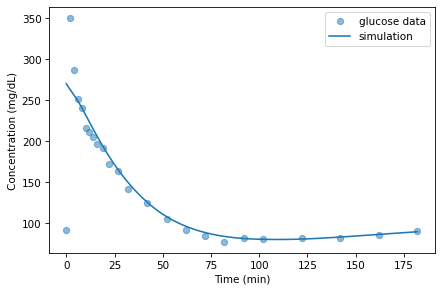
_images/4d008afbfc4169369e248d1b9f689a8ff745af0112c64e238161e7d1abe3c23b.png

With the parameters I chose, the model fits the data well except during the first few minutes after the injection. But we don’t expect the model to do well in this part of the time series.

The problem is that the model is non-spatial; that is, it does not take into account different concentrations in different parts of the body. Instead, it assumes that the concentrations of glucose and insulin in blood, and insulin in tissue fluid, are the same throughout the body. This way of representing the body is known among experts as the “bag of blood” model.

Immediately after injection, it takes time for the injected glucose to circulate. During that time, we don’t expect a non-spatial model to be accurate. For this reason, we should not take the estimated value of G0 too seriously; it is useful for fitting the model, but not meant to correspond to a physical, measurable quantity.

The following plot shows simulated insulin levels in the hypothetical “remote compartment”, which is in unspecified units.

results.X.plot(color='C1', label='remote insulin')

decorate(xlabel='Time (min)', 
         ylabel='Concentration (arbitrary units)')

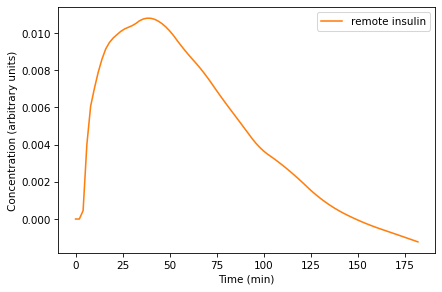
_images/f1f76fd16632cab190cf9428d118af4539d0373b8fc769008fb6ce494b7a7f50.png

Remember that X represents the concentration of insulin in the “remote compartment”, which is believed to be tissue fluid, so we can’t compare it to the measured concentration of insulin in the blood.

X rises quickly after the initial injection and then declines as the concentration of glucose declines. Qualitatively, this behavior is as expected, but because X is not an observable quantity, we can’t validate this part of the model quantitatively.

Solving Differential Equations#

To implement the minimal model, we rewrote the differential equations as difference equations with a finite time step, dt. When \(dt\) is very small, or more precisely infinitesimal, the difference equations are the same as the differential equations. But in our simulations, \(dt\) is 2 min, which is not very small, and definitely not infinitesimal.

In effect, the simulations assume that the derivatives \(dG/dt\) and \(dX/dt\) are constant during each 2 min time step. This method, evaluating derivatives at discrete time steps and assuming that they are constant in between, is called Euler’s method (see http://modsimpy.com/euler).

Euler’s method is good enough for many problems, but sometimes it is not very accurate. In that case, we can usually make it more accurate by decreasing the size of dt. But then it is not very efficient.

There are other methods that are more accurate and more efficient than Euler’s method. SciPy provides several of them wrapped in a function called solve_ivp. The ivp stands for initial value problem, which is the term for problems like the ones we’ve been solving, where we are given the initial conditions and try to predict what will happen.

The ModSim library provides a function called run_solve_ivp that makes solve_ivp a little easier to use.

To use it, we have to provide a slope function, which is similar to an update function; in fact, it takes the same parameters: a time stamp, a State object, and a System object.

Here’s a slope function that evaluates the differential equations of the minimal model.

def slope_func(t, state, system):
    G, X = state
    G0, k1, k2, k3 = system.params 
    I, Ib, Gb = system.I, system.Ib, system.Gb
        
    dGdt = -k1 * (G - Gb) - X*G
    dXdt = k3 * (I(t) - Ib) - k2 * X
    
    return dGdt, dXdt

slope_func is a little simpler than update_func because it computes only the derivatives, that is, the slopes. It doesn’t do the updates; the solver does them for us.

Now we can call run_solve_ivp like this:

results2, details = run_solve_ivp(system, slope_func,
                                  t_eval=results.index)

run_solve_ivp is similar to run_simulation: it takes a System object and a slope function as parameters.

The third argument, t_eval, is optional; it specifies where the solution should be evaluated.

It returns two values: a TimeFrame, which we assign to results2, and an OdeResult object, which we assign to details.

The OdeResult object contains information about how the solver ran, including a success code and a diagnostic message.

details.success

True

details.message

'The solver successfully reached the end of the integration interval.'

It’s important to check these messages after running the solver, in case anything went wrong.

The TimeFrame has one row for each time step and one column for each state variable. In this example, the rows are time from 0 to 182 minutes; the columns are the state variables, G and X. Here are the first few time steps:

results2.head()

	G	X
0.0	270.000000	0.000000
2.0	262.980942	0.000240
4.0	255.683455	0.002525
6.0	247.315442	0.005174
8.0	238.271851	0.006602

Because we used t_eval=results.index, the time stamps in results2 are the same as in results, which makes them easier to compare.

The following figure shows the results from run_solve_ivp along with the results from run_simulation:

results.G.plot(style='--', label='simulation')
results2.G.plot(style='-', label='solve ivp')

decorate(xlabel='Time (min)',
         ylabel='Concentration (mg/dL)')

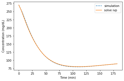
_images/3d388c5c0e40817c7b146145abf2ef4955b3d9c628e13c5651a2862b701c6499.png

The differences are barely visible. We can compute the relative differences like this:

diff = results.G - results2.G
percent_diff = diff / results2.G * 100

And we can use describe to compute summary statistics:

percent_diff.abs().describe()

count    92.000000
mean      0.649121
std       0.392903
min       0.000000
25%       0.274854
50%       0.684262
75%       1.009868
max       1.278168
Name: G, dtype: float64

The mean relative difference is about 0.65% and the maximum is a little more than 1%. Here are the results for X.

results.X.plot(style='--', label='simulation')
results2.X.plot(style='-', label='solve ivp')

decorate(xlabel='Time (min)', 
         ylabel='Concentration (arbitrary units)')

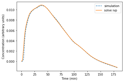
_images/a4e210e89e98d4176c0103bf7b450facacd08d46d898aaf1bd729ce2a060f488.png

These differences are a little bigger, especially at the beginning.

If we use run_simulation with smaller time steps, the results are more accurate, but they take longer to compute. For some problems, we can find a value of dt that produces accurate results in a reasonable time. However, if dt is too small, the results can be inaccurate again. So it can be tricky to get it right.

The advantage of run_solve_ivp is that it chooses the step size automatically in order to balance accuracy and efficiency. You can use keyword arguments to adjust this balance, but most of the time the results are accurate enough, and the computation is fast enough, without any intervention.

Summary#

In this chapter, we implemented the glucose minimal model two ways, using run_simulation and run_solve_ivp, and compared the results. We found that in this example, run_simulation, which uses Euler’s method, is probably good enough. But soon we will see examples where it is not.

So far, we have assumed that the parameters of the system are known, but in practice that’s not true. As one of the case studies in the next chapter, you’ll have a chance to see where those parameters came from.

Exercises#

This chapter is available as a Jupyter notebook where you can read the text, run the code, and work on the exercises. You can access the notebooks at https://allendowney.github.io/ModSimPy/.

Exercise 1#

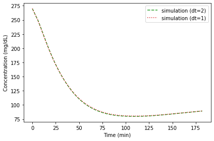
Our solution to the differential equations is only approximate because we used a finite step size, dt=2 minutes. If we make the step size smaller, we expect the solution to be more accurate. Run the simulation with dt=1 and compare the results. What is the largest relative error between the two solutions?