Torque

Torque#

This chapter is available as a Jupyter notebook where you can read the text, run the code, and work on the exercises. Click here to access the notebooks: https://allendowney.github.io/ModSimPy/.

In the previous chapter we modeled a system with constant angular velocity. In this chapter we take the next step, modeling a system with angular acceleration and deceleration.

Angular Acceleration#

Just as linear acceleration is the derivative of velocity, angular acceleration is the derivative of angular velocity. And just as linear acceleration is caused by force, angular acceleration is caused by the rotational version of force, torque. If you are not familiar with torque, you can read about it at http://modsimpy.com/torque.

In general, torque is a vector quantity, defined as the cross product of \(\vec{r}\) and \(\vec{F}\), where \(\vec{r}\) is the lever arm, a vector from the center of rotation to the point where the force is applied, and \(\vec{F}\) is the vector that represents the magnitude and direction of the force.

For the problems in this chapter, however, we only need the magnitude of torque; we don’t care about the direction. In that case, we can compute this product of scalar quantities:

\[\tau = r F \sin \theta\]

where \(\tau\) is torque, \(r\) is the length of the lever arm, \(F\) is the magnitude of force, and \(\theta\) is the angle between \(\vec{r}\) and \(\vec{F}\).

Since torque is the product of a length and a force, it is expressed in newton meters (Nm).

Moment of Inertia#

In the same way that linear acceleration is related to force by Newton’s second law of motion, \(F=ma\), angular acceleration is related to torque by another form of Newton’s law:

\[\tau = I \alpha\]

where \(\alpha\) is angular acceleration and \(I\) is moment of inertia. Just as mass is what makes it hard to accelerate an object, moment of inertia is what makes it hard to spin an object.

In the most general case, a 3-D object rotating around an arbitrary axis, moment of inertia is a tensor, which is a function that takes a vector as a parameter and returns a vector as a result.

Fortunately, in a system where all rotation and torque happens around a single axis, we don’t have to deal with the most general case. We can treat moment of inertia as a scalar quantity.

For a small object with mass \(m\), rotating around a point at distance \(r\), the moment of inertia is \(I = m r^2\). For more complex objects, we can compute \(I\) by dividing the object into small masses, computing moments of inertia for each mass, and adding them up. For most simple shapes, people have already done the calculations; you can just look up the answers. For example, see http://modsimpy.com/moment.

Teapots and Turntables#

Tables in Chinese restaurants often have a rotating tray or turntable that makes it easy for customers to share dishes. These turntables are supported by low-friction bearings that allow them to turn easily and glide. However, they can be heavy, especially when they are loaded with food, so they have a high moment of inertia.

Suppose I am sitting at a table with a pot of tea on the turntable directly in front of me, and the person sitting directly opposite asks me to pass the tea. I push on the edge of the turntable with 2 N of force until it has turned 0.5 rad, then let go. The turntable glides until it comes to a stop 1.5 rad from the starting position. How much force should I apply for a second push so the teapot glides to a stop directly opposite me?

We’ll answer this question in these steps:

I’ll use the results from the first push to estimate the coefficient of friction for the turntable.
As an exercise, you’ll use that coefficient of friction to estimate the force needed to rotate the turntable through the remaining angle.

Our simulation will use the following parameters:

The radius of the turntable is 0.5 m, and its weight is 7 kg.
The teapot weights 0.3 kg, and it sits 0.4 m from the center of the turntable.

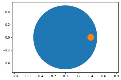
The following figure shows the scenario, where \(F\) is the force I apply to the turntable at the perimeter, perpendicular to the lever arm, \(r\), and \(\tau\) is the resulting torque. The circle near the bottom is the teapot.

Diagram of a turntable with ateapot.

Here are the parameters from the statement of the problem:

from numpy import pi

radius_disk = 0.5     # m
mass_disk = 7         # kg
radius_pot = 0.4      # m
mass_pot = 0.3        # kg
force = 2             # N

theta_push = 0.5        # radian
theta_test = 1.5        # radian
theta_target = pi       # radian

theta_push is the angle where I stop pushing on the turntable. theta_test is how far the table turns during my test push. theta_target is where we want the table to be after the second push.

We can use these parameters to compute the moment of inertia of the turntable, using the formula for a horizontal disk revolving around a vertical axis through its center:

I_disk = mass_disk * radius_disk**2 / 2

We can also compute the moment of inertia of the teapot, treating it as a point mass:

I_pot = mass_pot * radius_pot**2

The total moment of inertia is the sum of these parts:

I_total = I_disk + I_pot

Friction in the bearings probably depends on the weight of the turntable and its contents, but probably does not depend on angular velocity. So we’ll assume that it is a constant. We don’t know what it is, so I will start with a guess, and we will use root_scalar to improve it.

torque_friction = 0.3   # N*m

For this problem we’ll treat friction as a torque.

The state variables we’ll use are theta, which is the angle of the table in rad, and omega, which is angular velocity in rad/s.

init = State(theta=0, omega=0)

Now we can make a System with the initial state, init, the maximum duration of the simulation, t_end, and the parameters we are going to vary, force and torque_friction.

system = System(init=init, 
                force=force,
                torque_friction=torque_friction,
                t_end=20)

Here’s a slope function that takes the current state, which contains angle and angular velocity, and returns the derivatives, angular velocity and angular acceleration:

def slope_func(t, state, system):
    theta, omega = state
    force = system.force
    torque_friction = system.torque_friction
    
    torque = radius_disk * force - torque_friction
    alpha = torque / I_total
    
    return omega, alpha 

In this scenario, the force I apply to the turntable is always perpendicular to the lever arm, so \(\sin \theta = 1\) and the torque due to force is \(\tau = r F\).

torque_friction represents the torque due to friction. Because the turntable is rotating in the direction of positive theta, friction acts in the direction of negative theta.

We can test the slope function with the initial conditions:

slope_func(0, system.init, system)

(0, 0.7583965330444203)

We are almost ready to run the simulation, but first there’s a problem we have to address.

Two Phase Simulation#

When I stop pushing on the turntable, the angular acceleration changes abruptly. We could implement the slope function with an if statement that checks the value of theta and sets force accordingly. And for a coarse model like this one, that might be fine. But a more robust approach is to simulate the system in two phases:

During the first phase, force is constant, and we run until theta is 0.5 radians.
During the second phase, force is 0, and we run until omega is 0.

Then we can combine the results of the two phases into a single TimeFrame.

Phase 1#

Here’s the event function I’ll use for Phase 1; it stops the simulation when theta reaches theta_push, which is when I stop pushing:

def event_func1(t, state, system):
    theta, omega = state
    return theta - theta_push

We can test it with the initial conditions.

event_func1(0, system.init, system)

-0.5

And run the first phase of the simulation.

results1, details1 = run_solve_ivp(system, slope_func,
                                   events=event_func1)
details1.message

'A termination event occurred.'

Here are the last few time steps.

results1.tail()

	theta	omega
1.102359	0.46080	0.836025
1.113842	0.47045	0.844734
1.125325	0.48020	0.853442
1.136808	0.49005	0.862151
1.148291	0.50000	0.870860

It takes a little more than a second for me to rotate the table 0.5 rad. When I release the table, the angular velocity is about 0.87 rad / s.

Before we run the second phase, we have to extract the final time and state of the first phase.

t_2 = results1.index[-1]
init2 = results1.iloc[-1]

Phase 2#

Now we can make a System object for Phase 2 with the initial state from Phase 1 and with force=0.

system2 = system.set(t_0=t_2, init=init2, force=0)

For the second phase, we need an event function that stops when the turntable stops; that is, when angular velocity is 0.

def event_func2(t, state, system):
    theta, omega = state
    return omega

We’ll test it with the initial conditions for Phase 2.

event_func2(system2.t_0, system2.init, system2)

0.8708596517490182

The result is the angular velocity at the beginning of Phase 2, in rad/s.

Now we can run the second phase.

results2, details2 = run_solve_ivp(system2, slope_func,
                                   events=event_func2)
details2.message

'A termination event occurred.'

Combining the Results#

Pandas provides a function called concat, which makes a DataFrame with the rows from results1 followed by the rows from results2.

results = pd.concat([results1, results2])

Here are the last few time steps.

results.tail()

	theta	omega
3.720462	1.664800	3.483439e-02
3.747255	1.665617	2.612579e-02
3.774049	1.666200	1.741719e-02
3.800842	1.666550	8.708597e-03
3.827636	1.666667	-2.220446e-16

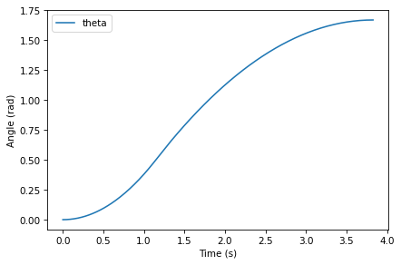
At the end, angular velocity is close to 0, and the total rotation is about 1.7 rad, a little farther than we were aiming for.

We can plot theta for both phases.

results.theta.plot(label='theta')
decorate(xlabel='Time (s)',
             ylabel='Angle (rad)')

_images/1876f5c3fe769123eaeb45a13314f9bb708d3dac21d39e835a4454ce961a24a6.png

And omega.

results.omega.plot(label='omega', color='C1')
decorate(xlabel='Time (s)',
             ylabel='Angular velocity (rad/s)')

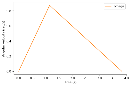
_images/546cf1c2f0b14aa2c733748c44bc02e5f912fa3cdf8c7f754c615289a3cb2f97.png

Angular velocity, omega, increases linearly while I am pushing, and decreases linearly after I let go. The angle, theta, is the integral of angular velocity, so it forms a parabola during each phase.

In the next section, we’ll use this simulation to estimate the torque due to friction.

Estimating Friction#

Let’s take the code from the previous section and wrap it in a function.

def run_two_phases(force, torque_friction, system):
    
    # put the specified parameters into the System object
    system1 = system.set(force=force, 
                         torque_friction=torque_friction)

    # run phase 1
    results1, details1 = run_solve_ivp(system1, slope_func, 
                                       events=event_func1)

    # get the final state from phase 1
    t_2 = results1.index[-1]
    init2 = results1.iloc[-1]
    
    # run phase 2
    system2 = system1.set(t_0=t_2, init=init2, force=0)
    results2, details2 = run_solve_ivp(system2, slope_func, 
                                       events=event_func2)
    
    # combine and return the results
    results = pd.concat([results1, results2])
    return results

I’ll test it with the same parameters.

force = 2
torque_friction = 0.3
results = run_two_phases(force, torque_friction, system)
results.tail()

	theta	omega
3.720462	1.664800	3.483439e-02
3.747255	1.665617	2.612579e-02
3.774049	1.666200	1.741719e-02
3.800842	1.666550	8.708597e-03
3.827636	1.666667	-2.220446e-16

These results are the same as in the previous section.

We can use run_two_phases to write an error function we can use, with root_scalar, to find the torque due to friction that yields the observed results from the first push, a total rotation of 1.5 rad.

def error_func1(torque_friction, system):
    force = system.force
    results = run_two_phases(force, torque_friction, system)
    theta_final = results.iloc[-1].theta
    print(torque_friction, theta_final)
    return theta_final - theta_test

This error function takes torque due to friction as an input. It extracts force from the System object and runs the simulation. From the results, it extracts the last value of theta and returns the difference between the result of the simulation and the result of the experiment. When this difference is 0, the value of torque_friction is an estimate for the friction in the experiment.

To bracket the root, we need one value that’s too low and one that’s too high. With torque_friction=0.3, the table rotates a bit too far:

guess1 = 0.3
error_func1(guess1, system)

0.3 1.666666666666669

0.16666666666666896

With torque_friction=0.4, it doesn’t go far enough.

guess2 = 0.4
error_func1(guess2, system)

0.4 1.2499999999999996

-0.25000000000000044

So we can use those two values as a bracket for root_scalar.

res = root_scalar(error_func1, system, bracket=[guess1, guess2])

3 1.666666666666669
3 1.666666666666669
4 1.2499999999999996
3400000000000003 1.4705882352941169
3340000000000002 1.4970059880239517
3333320000000001 1.5000060000239976
3333486666010001 1.4999310034693254

The result is 0.333 N m, a little less than the initial guess.

actual_friction = res.root
actual_friction

0.3333320000000001

Now that we know the torque due to friction, we can compute the force needed to rotate the turntable through the remaining angle, that is, from 1.5 rad to 3.14 rad. You’ll have a chance to do that as an exercise, but first, let’s animate the results.

Animating the Turntable#

Here’s a function that takes the state of the system and draws it.

from matplotlib.patches import Circle
from matplotlib.pyplot import gca, axis

def draw_func(t, state):
    theta, omega = state
    
    # draw a circle for the table
    circle1 = Circle([0, 0], radius_disk)
    gca().add_patch(circle1)
    
    # draw a circle for the teapot
    center = pol2cart(theta, radius_pot)
    circle2 = Circle(center, 0.05, color='C1')
    gca().add_patch(circle2)

    axis('equal')

This function uses a few features we have not seen before, but you can read about them in the Matplotlib documentation.

Here’s what the initial condition looks like.

state = results.iloc[0]
draw_func(0, state)

_images/47137779ab26692c5c30a8f0164296b9b7f871a54b46b22fc94744d0fc271871.png

And here’s how we call it.

# animate(results, draw_func)

Summary#

The example in this chapter demonstrates the concepts of torque, angular acceleration, and moment of inertia. We used these concepts to simulate a turntable, using a hypothetical observation to estimate torque due to friction. As an exercise, you can finish off the example, estimating the force needed to rotate the table to a given target angle.

The next chapter describes several case studies you can work on to practice the tools from the last few chapters, including projectiles, rotating objects, root_scalar, and maximize_scalar.

Exercises#

This chapter is available as a Jupyter notebook where you can read the text, run the code, and work on the exercises. You can access the notebooks at https://allendowney.github.io/ModSimPy/.

Exercise 1#

Continuing the example from this chapter, estimate the force that delivers the teapot to the desired position. Use this System object, with the friction we computed in the previous section.

system3 = system.set(torque_friction=actual_friction)

Write an error function that takes force and system, simulates the system, and returns the difference between theta_final and the remaining angle after the first push.

remaining_angle = theta_target - theta_test
remaining_angle

1.6415926535897931

Use your error function and root_scalar to find the force needed for the second push. Run the simulation with the force you computed and confirm that the table stops at the target angle after both pushes.