Proportional Growth

Proportional Growth#

This chapter is available as a Jupyter notebook where you can read the text, run the code, and work on the exercises. Click here to access the notebooks: https://allendowney.github.io/ModSimPy/.

In the previous chapter we simulated a model of world population with constant growth. In this chapter we’ll see if we can make a better model with growth proportional to the population.

But first, we’ll improve the code from the previous chapter by encapsulating it in a function and adding a new feature, a System object.

System Objects#

Like a State object, a System object contains variables and their values. The difference is:

State objects contain state variables that get updated in the course of a simulation.
System objects contain system parameters, which usually don’t get updated over the course of a simulation.

For example, in the bike share model, state variables include the number of bikes at each location, which get updated whenever a customer moves a bike. System parameters include the number of locations, total number of bikes, and arrival rates at each location.

In the population model, the only state variable is the population. System parameters include the annual growth rate, the initial population, and the start and end times.

Suppose we have the following variables, as computed in the previous chapter (assuming table2 is the DataFrame we read from the file):

un = table2.un / 1e9
census = table2.census / 1e9

t_0 = census.index[0]
t_end = census.index[-1]
elapsed_time = t_end - t_0

p_0 = census[t_0]
p_end = census[t_end]

total_growth = p_end - p_0
annual_growth = total_growth / elapsed_time

Some of these are parameters we need to simulate the system; others are temporary values we can discard. To distinguish between them, we’ll put the parameters we need in a System object like this:

system = System(t_0=t_0, 
                t_end=t_end,
                p_0=p_0,
                annual_growth=annual_growth)

t0 and t_end are the first and last years; p_0 is the initial population, and annual_growth is the estimated annual growth.

The assignment t_0=t_0 reads the value of the existing variable named t_0, which we created previously, and stores it in a new system variable, also named t_0. The variables inside the System object are distinct from other variables, so you can change one without affecting the other, even if they have the same name.

So this System object contains four new variables; here’s what they look like.

show(system)

	value
t_0	1950.000000
t_end	2016.000000
p_0	2.557629
annual_growth	0.072248

Next we’ll wrap the code from the previous chapter in a function:

def run_simulation1(system):
    results = TimeSeries()
    results[system.t_0] = system.p_0
    
    for t in range(system.t_0, system.t_end):
        results[t+1] = results[t] + system.annual_growth
    
    return results

run_simulation1 takes a System object and reads from it the values of t_0, t_end, and annual_growth.

It simulates population growth over time and returns the results in a TimeSeries. Here’s how we call it.

results1 = run_simulation1(system)

Here’s the function we used in the previous chapter to plot the estimates.

def plot_estimates():
    census.plot(style=':', label='US Census')
    un.plot(style='--', label='UN DESA')
    decorate(xlabel='Year', 
             ylabel='World population (billion)') 

And here are the results.

results1.plot(label='model', color='gray')
plot_estimates()
decorate(title='Constant growth model')

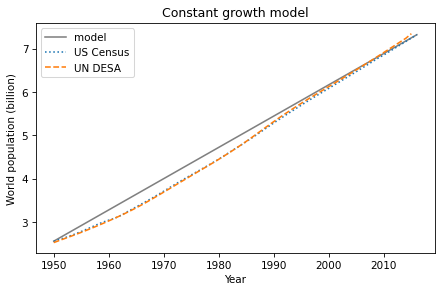
_images/2888bbbf035b4cf5e53c0c9e95ad14b6334a847807e99162fc9a4f2e9253f35f.png

It might not be obvious that using functions and System objects is a big improvement, and for a simple model that we run only once, maybe it’s not. But as we work with more complex models, and when we run many simulations with different parameters, we’ll see that this way of organizing the code makes a big difference.

Now let’s see if we can improve the model.

Proportional Growth Model#

The biggest problem with the constant growth model is that it doesn’t make any sense. It is hard to imagine how people all over the world could conspire to keep population growth constant from year to year.

On the other hand, if some fraction of the population dies each year, and some fraction gives birth, we can compute the net change in the population like this:

def run_simulation2(system):
    results = TimeSeries()
    results[system.t_0] = system.p_0
    
    for t in range(system.t_0, system.t_end):
        births = system.birth_rate * results[t]
        deaths = system.death_rate * results[t]
        results[t+1] = results[t] + births - deaths
        
    return results

Each time through the loop, we use the parameter birth_rate to compute the number of births, and death_rate to compute the number of deaths. The rest of the function is the same as run_simulation1.

Now we can choose the values of birth_rate and death_rate that best fit the data. For the death rate, I’ll use 7.7 deaths per 1000 people, which was roughly the global death rate in 2020 (see https://www.indexmundi.com/world/death_rate.html). I chose the birth rate by hand to fit the population data.

system.death_rate = 7.7 / 1000
system.birth_rate = 25 / 1000

Then I ran the simulation and plotted the results:

results2 = run_simulation2(system)
results2.plot(label='model', color='gray')
plot_estimates()
decorate(title='Proportional growth model')

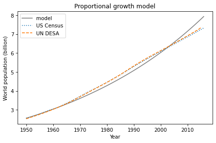
_images/e6ee74f84aaef6523358ec5a9503ab54c5eb6dfa8c06ccabd52edb5e1ef478ae.png

The proportional model fits the data well from 1950 to 1965, but not so well after that. Overall, the quality of fit is not as good as the constant growth model, which is surprising, because it seems like the proportional model is more realistic.

In the next chapter we’ll try one more time to find a model that makes sense and fits the data. But first, I want to make a few more improvements to the code.

Factoring Out the Update Function#

run_simulation1 and run_simulation2 are nearly identical except for the body of the for loop, where we compute the population for the next year.

Rather than repeat identical code, we can separate the things that change from the things that don’t. First, I’ll pull out the births and deaths from run_simulation2 and make a function:

def growth_func1(t, pop, system):
    births = system.birth_rate * pop
    deaths = system.death_rate * pop
    return births - deaths

growth_func1 takes as arguments the current year, current population, and a System object; it returns the net population growth during the current year.

This function does not use t, so we could leave it out. But we will see other growth functions that need it, and it is convenient if they all take the same parameters, used or not. Now we can write a function that runs any model:

def run_simulation(system, growth_func):
    results = TimeSeries()
    results[system.t_0] = system.p_0
    
    for t in range(system.t_0, system.t_end):
        growth = growth_func(t, results[t], system)
        results[t+1] = results[t] + growth
        
    return results

This function demonstrates a feature we have not seen before: it takes a function as a parameter! When we call run_simulation, the second parameter is a function, like growth_func1, that computes the population for the next year.

Here’s how we call it:

results = run_simulation(system, growth_func1)

Passing a function as an argument is the same as passing any other value. The argument, which is growth_func1 in this example, gets assigned to the parameter, which is called growth_func. Inside run_simulation, we can call growth_func just like any other function.

Each time through the loop, run_simulation calls growth_func1 to compute net growth, and uses it to compute the population during the next year.

Combining Birth and Death#

We can simplify the code slightly by combining births and deaths to compute the net growth rate. Instead of two parameters, birth_rate and death_rate, we can write the update function in terms of a single parameter that represents the difference:

system.alpha = system.birth_rate - system.death_rate

The name of this parameter, alpha, is the conventional name for a proportional growth rate.

Here’s the modified version of growth_func1:

def growth_func2(t, pop, system):
    return system.alpha * pop

And here’s how we run it:

results = run_simulation(system, growth_func2)

The results are the same as the previous versions, but now the code is organized in a way that makes it easy to explore other models.

Summary#

In this chapter, we wrapped the code from the previous chapter in functions and used a System object to store the parameters of the system.

We explored a new model of population growth, where the number of births and deaths is proportional to the current population. This model seems more realistic, but it turns out not to fit the data particularly well.

In the next chapter, we’ll try one more model, which is based on the assumption that the population can’t keep growing forever. But first, you might want to work on some exercises.

Exercises#

Exercise 1#

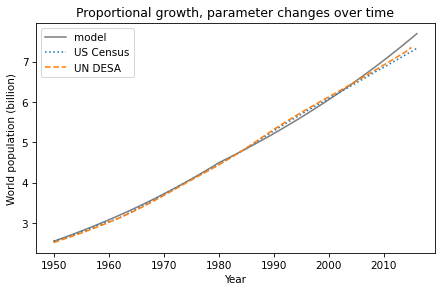
Maybe the reason the proportional model doesn’t work very well is that the growth rate, alpha, is changing over time. So let’s try a model with different growth rates before and after 1980 (as an arbitrary choice).

Write an update function that takes t, pop, and system as parameters. The system object, system, should contain two parameters: the growth rate before 1980, alpha1, and the growth rate after 1980, alpha2. It should use t to determine which growth rate to use.

Test your function by calling it directly, then pass it to run_simulation. Plot the results. Adjust the parameters alpha1 and alpha2 to fit the data as well as you can.

Under the Hood#

The System object defined in the ModSim library, is based on the SimpleNamespace object defined in a standard Python library called types; the documentation is at https://docs.python.org/3.7/library/types.html#types.SimpleNamespace.