Limits to Growth

Limits to Growth#

This chapter is available as a Jupyter notebook where you can read the text, run the code, and work on the exercises. Click here to access the notebooks: https://allendowney.github.io/ModSimPy/.

In the previous chapter we developed a population model where net growth during each time step is proportional to the current population. This model seems more realistic than the constant growth model, but it does not fit the data as well.

There are a few things we could try to improve the model:

Maybe net growth depends on the current population, but the relationship is quadratic, not linear.
Maybe the net growth rate varies over time.

In this chapter, we’ll explore the first option. In the exercises, you will have a chance to try the second.

Quadratic Growth#

It makes sense that net growth should depend on the current population, but maybe it’s not a linear relationship, like this:

net_growth = system.alpha * pop

Maybe it’s a quadratic relationship, like this:

net_growth = system.alpha * pop + system.beta * pop**2

We can test that conjecture with a new update function:

def growth_func_quad(t, pop, system):
    return system.alpha * pop + system.beta * pop**2

Here’s the System object we’ll use, initialized with t_0, p_0, and t_end.

t_0 = census.index[0]
p_0 = census[t_0]
t_end = census.index[-1]

system = System(t_0=t_0,
                p_0=p_0,
                t_end=t_end)

Now we have to add the parameters alpha and beta . I chose the following values by trial and error; we’ll see better ways to do it later.

system.alpha = 25 / 1000
system.beta = -1.8 / 1000

And here’s how we run it:

results = run_simulation(system, growth_func_quad)

Here are the results.

results.plot(color='gray', label='model')
plot_estimates()
decorate(title='Quadratic growth model')

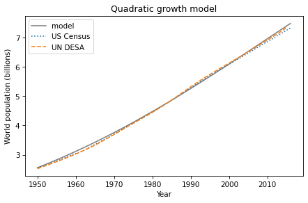
_images/2afa50d9318074dd26999ccad4fd51ef8a28e54914ebc850ea263e4fdebf43b9.png

The model fits the data well over the whole range, with just a bit of space between them in the 1960s.

It is not entirely surprising that the quadratic model fits better than the constant and proportional models, because it has two parameters we can choose, where the other models have only one. In general, the more parameters you have to play with, the better you should expect the model to fit.

But fitting the data is not the only reason to think the quadratic model might be a good choice. It also makes sense; that is, there is a legitimate reason to expect the relationship between growth and population to have this form.

To understand it, let’s look at net growth as a function of population.

Net Growth#

Let’s plot the relationship between growth and population in the quadratic model. I’ll use linspace to make an array of 101 populations from 0 to 15 billion.

from numpy import linspace

pop_array = linspace(0, 15, 101)

Now I’ll use the quadratic model to compute net growth for each population.

growth_array = (system.alpha * pop_array + 
                system.beta * pop_array**2)

To plot growth rate versus population, we’ll use the plot function from Matplotlib. First we have to import it:

from matplotlib.pyplot import plot

Now we can use it like this:

plot(pop_array, growth_array, label='net growth', color='C2')

decorate(xlabel='Population (billions)',
         ylabel='Net growth (billions)',
         title='Net growth vs. population')

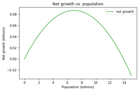
_images/76d0b47d2df8a43d9cca38b8c3cb1736ec1f49baff5d930dd7865f8cc751fd4d.png

Note that the x-axis is not time, as in the previous figures, but population. We can divide this curve into four kinds of behavior:

When the population is less than 3 billion, net growth is proportional to population, as in the proportional model. In this range, the population grows slowly because the population is small.
Between 3 billion and 10 billion, the population grows quickly because there are a lot of people.
Above 10 billion, population grows more slowly; this behavior models the effect of resource limitations that decrease birth rates or increase death rates.
Above 14 billion, resources are so limited that the death rate exceeds the birth rate and net growth becomes negative.

Just below 14 billion, there is a point where net growth is 0, which means that the population does not change. At this point, the birth and death rates are equal, so the population is in equilibrium.

Finding Equilibrium#

The equilibrium point is the population, \(p\), where net population growth, \(\Delta p\), is 0. We can compute it by finding the roots, or zeros, of this equation:

\[\Delta p = \alpha p + \beta p^2\]

where \(\alpha\) and \(\beta\) are the parameters of the model. If we rewrite the right-hand side like this:

\[\Delta p = p (\alpha + \beta p)\]

we can see that net growth is \(0\) when \(p=0\) or \(p=-\alpha/\beta\). So we can compute the (non-zero) equilibrium point like this:

-system.alpha / system.beta

13.88888888888889

With these parameters, net growth is 0 when the population is about 13.9 billion (the result is positive because beta is negative).

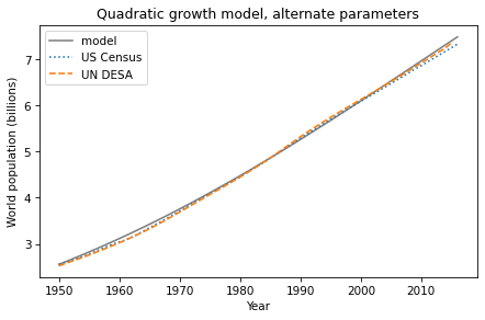
In the context of population modeling, the quadratic model is more conventionally written like this:

\[\Delta p = r p (1 - p / K)\]

This is the same model; it’s just a different way to parameterize it. Given \(\alpha\) and \(\beta\), we can compute \(r=\alpha\) and \(K=-\alpha/\beta\).

In this version, it is easier to interpret the parameters: \(r\) is the unconstrained growth rate, observed when \(p\) is small, and \(K\) is the equilibrium point. \(K\) is also called the carrying capacity, since it indicates the maximum population the environment can sustain.

Summary#

In this chapter we implemented a quadratic growth model where net growth depends on the current population and the population squared. This model fits the data well, and we saw one reason why: it is based on the assumption that there is a limit to the number of people the Earth can support.

In the next chapter we’ll use the models we have developed to generate predictions. But first, I want to warn you about a few things that can go wrong when you write functions.

Dysfunctions#

When people learn about functions, there are a few things they often find confusing. In this section I’ll present and explain some common problems.

As an example, suppose you want a function that takes a System object, with variables alpha and beta, and computes the carrying capacity, -alpha/beta. Here’s a good solution:

def carrying_capacity(system):
    K = -system.alpha / system.beta
    return K
    
sys1 = System(alpha=0.025, beta=-0.0018)
pop = carrying_capacity(sys1)
print(pop)

13.88888888888889

Now let’s see all the ways that can go wrong.

Dysfunction #1: Not using parameters. In the following version, the function doesn’t take any parameters; when sys1 appears inside the function, it refers to the object we create outside the function.

def carrying_capacity():
    K = -sys1.alpha / sys1.beta
    return K
    
sys1 = System(alpha=0.025, beta=-0.0018)
pop = carrying_capacity()
print(pop)

13.88888888888889

This version works, but it is not as versatile as it could be. If there are several System objects, this function can work with only one of them, and only if it is named sys1.

Dysfunction #2: Clobbering the parameters. When people first learn about parameters, they often write functions like this:

# WRONG
def carrying_capacity(system):
    system = System(alpha=0.025, beta=-0.0018)
    K = -system.alpha / system.beta
    return K
    
sys1 = System(alpha=0.03, beta=-0.002)
pop = carrying_capacity(sys1)
print(pop)

13.88888888888889

In this example, we have a System object named sys1 that gets passed as an argument to carrying_capacity. But when the function runs, it ignores the argument and immediately replaces it with a new System object. As a result, this function always returns the same value, no matter what argument is passed.

When you write a function, you generally don’t know what the values of the parameters will be. Your job is to write a function that works for any valid values. If you assign your own values to the parameters, you defeat the whole purpose of functions.

Dysfunction #3: No return value. Here’s a version that computes the value of K but doesn’t return it.

# WRONG
def carrying_capacity(system):
    K = -system.alpha / system.beta
    
sys1 = System(alpha=0.025, beta=-0.0018)
pop = carrying_capacity(sys1)
print(pop)

None

A function that doesn’t have a return statement actually returns a special value called None, so in this example the value of pop is None. If you are debugging a program and find that the value of a variable is None when it shouldn’t be, a function without a return statement is a likely cause.

Dysfunction #4: Ignoring the return value. Finally, here’s a version where the function is correct, but the way it’s used is not.

def carrying_capacity(system):
    K = -system.alpha / system.beta
    return K
    
sys1 = System(alpha=0.025, beta=-0.0018)
carrying_capacity(sys1)   # WRONG
print(K)

In this example, carrying_capacity runs and returns K, but the return value doesn’t get displayed or assigned to a variable. If we try to print K, we get a NameError, because K only exists inside the function.

When you call a function that returns a value, you should do something with the result.

Exercises#

Exercise 1#

In a previous section, we saw a different way to parameterize the quadratic model:

\[ \Delta p = r p (1 - p / K) \]

where \(r=\alpha\) and \(K=-\alpha/\beta\).

Write a version of growth_func that implements this version of the model. Test it by computing the values of r and K that correspond to alpha=0.025 and beta=-0.0018, and confirm that you get the same results.

Exercise 2#

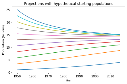
What happens if we start with an initial population above the carrying capacity, like 20 billion? Run the model with initial populations between 1 and 20 billion, and plot the results on the same axes.

Hint: If there are too many labels in the legend, you can plot results like this:

    results.plot(label='_nolegend')