Printed and electronic copies of Modeling and Simulation in Python are available from No Starch Press and Bookshop.org and Amazon.
Epidemiology#
In this chapter, we’ll develop a model of an epidemic as it spreads in a susceptible population, and use it to evaluate the effectiveness of possible interventions.
My presentation of the model in the next few chapters is based on an excellent article by David Smith and Lang Moore, “The SIR Model for Spread of Disease,” Journal of Online Mathematics and its Applications, December 2001, available at http://modsimpy.com/sir.
The Freshman Plague#
Every year at Olin College, about 90 new students come to campus from around the country and the world. Most of them arrive healthy and happy, but usually at least one brings with them some kind of infectious disease. A few weeks later, predictably, some fraction of the incoming class comes down with what we call the “Freshman Plague”.
In this chapter we introduce a well-known model of infectious disease, the Kermack-McKendrick model, and use it to explain the progression of the disease over the course of the semester, predict the effect of possible interventions (like immunization) and design the most effective intervention campaign.
So far we have done our own modeling; that is, we’ve chosen physical systems, identified factors that seem important, and made decisions about how to represent them. In this chapter we start with an existing model and reverse-engineer it. Along the way, we consider the modeling decisions that went into it and identify its capabilities and limitations.
The Kermack-McKendrick Model#
The Kermack-McKendrick (KM) model is an example of an SIR model, so-named because it represents three categories of people:
S: People who are “susceptible”, that is, capable of contracting the disease if they come into contact with someone who is infected.
I: People who are “infectious”, that is, capable of passing along the disease if they come into contact with someone susceptible.
R: People who are “recovered”. In the basic version of the model, people who have recovered are considered to be no longer infectious and immune to reinfection. That is a reasonable model for some diseases, but not for others, so it should be on the list of assumptions to reconsider later.
Let’s think about how the number of people in each category changes over time. Suppose we know that people with the disease are infectious for a period of 4 days, on average. If 100 people are infectious at a particular point in time, and we ignore the particular time each one became infected, we expect about 1 out of 4 to recover on any particular day.
Putting that a different way, if the time between recoveries is 4 days, the recovery rate is about 0.25 recoveries per day, which we’ll denote with the Greek letter gamma, \(\gamma\), or the variable name gamma.
If the total number of people in the population is \(N\), and the fraction currently infectious is \(i\), the total number of recoveries we expect per day is \(\gamma i N\).
Now let’s think about the number of new infections. Suppose we know that each susceptible person comes into contact with 1 person every 3 days, on average, in a way that would cause them to become infected if the other person is infected. We’ll denote this contact rate with the Greek letter beta, \(\beta\), or the variables name beta.
It’s probably not reasonable to assume that we know \(\beta\) ahead of time, but later we’ll see how to estimate it based on data from previous outbreaks.
If \(s\) is the fraction of the population that’s susceptible, \(s N\) is the number of susceptible people, \(\beta s N\) is the number of contacts per day, and \(\beta s i N\) is the number of those contacts where the other person is infectious.
In summary:
The number of recoveries we expect per day is \(\gamma i N\); dividing by \(N\) yields the fraction of the population that recovers in a day, which is \(\gamma i\).
The number of new infections we expect per day is \(\beta s i N\); dividing by \(N\) yields the fraction of the population that gets infected in a day, which is \(\beta s i\).
The KM model assumes that the population is closed; that is, no one arrives or departs, so the size of the population, \(N\), is constant.
The KM Equations#
If we treat time as a continuous quantity, we can write differential equations that describe the rates of change for \(s\), \(i\), and \(r\) (where \(r\) is the fraction of the population that has recovered):
To avoid cluttering the equations, I leave it implied that \(s\) is a function of time, \(s(t)\), and likewise for \(i\) and \(r\).
SIR models are examples of compartment models, so-called because they divide the world into discrete categories, or compartments, and describe transitions from one compartment to another. Compartments are also called stocks and transitions between them are called flows.
In this example, there are three stocks—susceptible, infectious, and recovered—and two flows—new infections and recoveries. Compartment models are often represented visually using stock and flow diagrams (see http://modsimpy.com/stock).
The following figure shows the stock and flow diagram for the KM model.

Stocks are represented by rectangles, flows by arrows. The widget in the middle of the arrows represents a valve that controls the rate of flow; the diagram shows the parameters that control the valves.
Implementing the KM model#
For a given physical system, there are many possible models, and for a given model, there are many ways to represent it. For example, we can represent an SIR model as a stock-and-flow diagram, as a set of differential equations, or as a Python program. The process of representing a model in these forms is called implementation. In this section, we implement the KM model in Python.
I’ll represent the initial state of the system using a State object
with state variables s, i, and r; they represent the fraction of
the population in each compartment.
We can initialize the State object with the number of people in each compartment; for example, here is the initial state with one infected student in a class of 90:
init = State(s=89, i=1, r=0)
show(init)
| state | |
|---|---|
| s | 89 |
| i | 1 |
| r | 0 |
We can convert the numbers to fractions by dividing by the total:
init /= init.sum()
show(init)
| state | |
|---|---|
| s | 0.988889 |
| i | 0.011111 |
| r | 0.000000 |
For now, let’s assume we know the time between contacts and time between recoveries:
tc = 3             # time between contacts in days
tr = 4             # recovery time in days
We can use them to compute the parameters of the model:
beta = 1 / tc      # contact rate in per day
gamma = 1 / tr     # recovery rate in per day
I’ll use a System object to store the parameters and initial
conditions. The following function takes the system parameters and returns a new System object:
def make_system(beta, gamma):
    init = State(s=89, i=1, r=0)
    init /= init.sum()

    return System(init=init, t_end=7*14,
                  beta=beta, gamma=gamma)
The default value for t_end is 14 weeks, about the length of a
semester.
Here’s what the System object looks like.
system = make_system(beta, gamma)
show(system)
| value | |
|---|---|
| init | s 0.988889 i 0.011111 r 0.000000 Name... |
| t_end | 98 |
| beta | 0.333333 |
| gamma | 0.25 |
Now that we have object to represent the system and its state, we are ready for the update function.
The Update Function#
The purpose of an update function is to take the current state of a system and compute the state during the next time step. Here’s the update function we’ll use for the KM model:
def update_func(t, state, system):
    s, i, r = state.s, state.i, state.r

    infected = system.beta * i * s
    recovered = system.gamma * i

    s -= infected
    i += infected - recovered
    r += recovered

    return State(s=s, i=i, r=r)
update_func takes as parameters the current time, a State object, and a System object.
The first line unpacks the State object, assigning the values of the state variables to new variables with the same names.
This is an example of multiple assignment.
The left side is a sequence of variables; the right side is a sequence of expressions.
The values on the right side are assigned to the variables on the left side, in order.
By creating these variables, we avoid repeating state several times, which makes the code easier to read.
The update function computes infected and recovered as a fraction of the population, then updates s, i and r. The return value is a State that contains the updated values.
We can call update_func like this:
state = update_func(0, init, system)
show(state)
| state | |
|---|---|
| s | 0.985226 |
| i | 0.011996 |
| r | 0.002778 |
The result is the new State object.
You might notice that this version of update_func does not use one of its parameters, t. I include it anyway because update functions
sometimes depend on time, and it is convenient if they all take the same parameters, whether they need them or not.
Running the Simulation#
Now we can simulate the model over a sequence of time steps:
def run_simulation1(system, update_func):
    state = system.init

    for t in range(0, system.t_end):
        state = update_func(t, state, system)

    return state
The parameters of run_simulation are the System object and the
update function. The System object contains the parameters, initial
conditions, and values of 0 and t_end.
We can call run_simulation like this:
final_state = run_simulation1(system, update_func)
show(final_state)
| state | |
|---|---|
| s | 0.520568 |
| i | 0.000666 |
| r | 0.478766 |
The result indicates that after 14 weeks (98 days), about 52% of the population is still susceptible, which means they were never infected, almost 48% have recovered, which means they were infected at some point, and less than 1% are actively infected.
Collecting the Results#
The previous version of run_simulation returns only the final state,
but we might want to see how the state changes over time. We’ll consider two ways to do that: first, using three TimeSeries objects, then using a new object called a TimeFrame.
Here’s the first version:
def run_simulation2(system, update_func):
    S = TimeSeries()
    I = TimeSeries()
    R = TimeSeries()

    state = system.init
    S[0], I[0], R[0] = state

    for t in range(0, system.t_end):
        state = update_func(t, state, system)
        S[t+1], I[t+1], R[t+1] = state.s, state.i, state.r

    return S, I, R
First, we create TimeSeries objects to store the results.
Next we initialize state and the first elements of S, I and
R.
Inside the loop, we use update_func to compute the state of the system at the next time step, then use multiple assignment to unpack the elements of state, assigning each to the corresponding TimeSeries.
At the end of the function, we return the values S, I, and R. This is the first example we have seen where a function returns more than one value.
We can run the function like this:
S, I, R = run_simulation2(system, update_func)
We’ll use the following function to plot the results:
def plot_results(S, I, R):
    S.plot(style='--', label='Susceptible')
    I.plot(style='-', label='Infected')
    R.plot(style=':', label='Recovered')
    decorate(xlabel='Time (days)',
             ylabel='Fraction of population')
And run it like this:
plot_results(S, I, R)
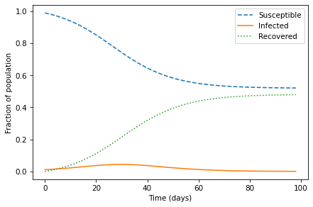
It takes about three weeks (21 days) for the outbreak to get going, and about five weeks (35 days) to peak. The fraction of the population that’s infected is never very high, but it adds up. In total, almost half the population gets sick.
Now With a TimeFrame#
If the number of state variables is small, storing them as separate
TimeSeries objects might not be so bad. But a better alternative is to use a TimeFrame, which is another object defined in the ModSim
library.
A TimeFrame is a kind of a DataFrame, which we used earlier to store world population estimates.
Here’s a more concise version of run_simulation using a TimeFrame:
def run_simulation(system, update_func):
    frame = TimeFrame(columns=system.init.index)
    frame.loc[0] = system.init

    for t in range(0, system.t_end):
        frame.loc[t+1] = update_func(t, frame.loc[t], system)

    return frame
The first line creates an empty TimeFrame with one column for each
state variable. Then, before the loop starts, we store the initial
conditions in the TimeFrame at 0. Based on the way we’ve been using
TimeSeries objects, it is tempting to write:
frame[0] = system.init
But when you use the bracket operator with a TimeFrame or DataFrame, it selects a column, not a row.
To select a row, we have to use loc, like this:
frame.loc[0] = system.init
Since the value on the right side is a State, the assignment matches
up the index of the State with the columns of the TimeFrame; that
is, it assigns the s value from system.init to the s column of
frame, and likewise with i and r.
Each time through the loop, we assign the State we get from update_func to the next row of frame.
At the end, we return frame.
We can call this version of run_simulation like this:
results = run_simulation(system, update_func)
Here are the first few rows of the results.
results.head()
| s | i | r | |
|---|---|---|---|
| 0 | 0.988889 | 0.011111 | 0.000000 |
| 1 | 0.985226 | 0.011996 | 0.002778 |
| 2 | 0.981287 | 0.012936 | 0.005777 |
| 3 | 0.977055 | 0.013934 | 0.009011 |
| 4 | 0.972517 | 0.014988 | 0.012494 |
The columns in the TimeFrame correspond to the state variables, s, i, and r.
As with a DataFrame, we can use the dot operator to select columns
from a TimeFrame, so we can plot the results like this:
plot_results(results.s, results.i, results.r)
The results are the same as before, now in a more convenient form.
Summary#
This chapter presents an SIR model of infectious disease and two ways to collect the results, using several TimeSeries objects or a single TimeFrame.
In the next chapter we’ll use the model to explore the effect of immunization.
But first you might want to work on these exercises.
Exercises#
This chapter is available as a Jupyter notebook where you can read the text, run the code, and work on the exercises. You can access the notebooks at https://allendowney.github.io/ModSimPy/.
Exercise 1#
Suppose the time between contacts is 4 days and the recovery time is 5 days. After 14 weeks, how many students, total, have been infected?
Hint: what is the change in S between the beginning and the end of the simulation?