Bike Share System

Bike Share System#

This chapter presents a simple model of a bike share system and demonstrates the features of Python we’ll use to develop simulations of real-world systems.

Along the way, we’ll make decisions about how to model the system. In the next chapter we’ll review these decisions and gradually improve the model.

This chapter is available as a Jupyter notebook where you can read the text, run the code, and work on the exercises. Click here to access the notebooks: https://allendowney.github.io/ModSimPy/.

Defining Functions#

So far we have used functions defined in NumPy and the ModSim library. Now we’re going to define our own functions.

When you are developing code in Jupyter, it is often efficient to write a few lines of code, test them to confirm they do what you intend, and then use them to define a new function. For example, these lines move a bike from Olin to Wellesley:

bikeshare.olin -= 1
bikeshare.wellesley += 1

Rather than repeat them every time a bike moves, we can define a new function:

def bike_to_wellesley():
    bikeshare.olin -= 1
    bikeshare.wellesley += 1

def is a special word in Python that indicates we are defining a new function. The name of the function is bike_to_wellesley. The empty parentheses indicate that this function requires no additional information when it runs. The colon indicates the beginning of an indented code block.

The next two lines are the body of the function. They have to be indented; by convention, the indentation is four spaces.

When you define a function, it has no immediate effect. The body of the function doesn’t run until you call the function. Here’s how to call this function:

bike_to_wellesley()

When you call the function, it runs the statements in the body, which update the variables of the bikeshare object; you can check by displaying the new state.

show(bikeshare)

	state
olin	6
wellesley	6

When you call a function, you have to include the parentheses. If you leave them out, you get this:

bike_to_wellesley

<function __main__.bike_to_wellesley()>

This result indicates that bike_to_wellesley is a function. You don’t have to know what __main__ means, but if you see something like this, it probably means that you named a function but didn’t actually call it. So don’t forget the parentheses.

Print Statements#

As you write more complicated programs, it is easy to lose track of what is going on. One of the most useful tools for debugging is the print statement, which displays text in the Jupyter notebook.

Normally when Jupyter runs the code in a cell, it displays the value of the last line of code. For example, if you run:

bikeshare.olin
bikeshare.wellesley

Jupyter runs both lines, but it only displays the value of the second. If you want to display more than one value, you can use print statements:

print(bikeshare.olin)
print(bikeshare.wellesley)

6
6

When you call the print function, you can put a variable in parentheses, as in the previous example, or you can provide a sequence of variables separated by commas, like this:

print(bikeshare.olin, bikeshare.wellesley)

6 6

Python looks up the values of the variables and displays them; in this example, it displays two values on the same line, with a space between them.

Print statements are useful for debugging functions. For example, we can add a print statement to bike_to_wellesley, like this:

def bike_to_wellesley():
    print('Moving a bike to Wellesley')
    bikeshare.olin -= 1
    bikeshare.wellesley += 1

Each time we call this version of the function, it displays a message, which can help us keep track of what the program is doing. The message in this example is a string, which is a sequence of letters and other symbols in quotes.

Just like bike_to_wellesley, we can define a function that moves a bike from Wellesley to Olin:

def bike_to_olin():
    print('Moving a bike to Olin')
    bikeshare.wellesley -= 1
    bikeshare.olin += 1

And call it like this:

bike_to_olin()

Moving a bike to Olin

One benefit of defining functions is that you avoid repeating chunks of code, which makes programs smaller. Another benefit is that the name you give the function documents what it does, which makes programs more readable.

If Statements#

At this point we have functions that simulate moving bikes; now let’s think about simulating customers. As a simple model of customer behavior, I will use a random number generator to determine when customers arrive at each station.

The ModSim library provides a function called flip that generates random “coin tosses”. When you call it, you provide a probability between 0 and 1, like this:

flip(0.7)

True

The result is one of two values: True with probability 0.7 (in this example) or False with probability 0.3. If you run flip like this 100 times, you should get True about 70 times and False about 30 times. But the results are random, so they might differ from these expectations.

True and False are special values defined by Python. They are called boolean values because they are related to Boolean algebra (https://modsimpy.com/boolean).

Note that they are not strings. There is a difference between True, which is a boolean value, and 'True', which is a string.

We can use boolean values to control the behavior of the program, using an if statement:

if flip(0.5):
    print('heads')

If the result from flip is True, the program displays the string 'heads'. Otherwise it does nothing.

The syntax for if statements is similar to the syntax for function definitions: the first line has to end with a colon, and the lines inside the if statement have to be indented.

Optionally, you can add an else clause to indicate what should happen if the result is False:

if flip(0.5):
    print('heads')
else:
    print('tails')    

heads

If you run the previous cell a few times, it should print heads about half the time, and tails about half the time.

Now we can use flip to simulate the arrival of customers who want to borrow a bike. Suppose students arrive at the Olin station every two minutes on average. In that case, the chance of an arrival during any one-minute period is 50%, and we can simulate it like this:

if flip(0.5):
    bike_to_wellesley()

Moving a bike to Wellesley

If students arrive at the Wellesley station every three minutes, on average, the chance of an arrival during any one-minute period is 33%, and we can simulate it like this:

if flip(0.33):
    bike_to_olin()

We can combine these snippets into a function that simulates a time step, which is an interval of time, in this case one minute:

def step():
    if flip(0.5):
        bike_to_wellesley()
    
    if flip(0.33):
        bike_to_olin()

Then we can simulate a time step like this:

step()

Depending on the results from flip, this function might move a bike to Olin, or to Wellesley, or neither, or both.

Parameters#

The previous version of step is fine if the arrival probabilities never change, but in reality they vary over time.

So instead of putting the constant values 0.5 and 0.33 in step, we can replace them with parameters. Parameters are variables whose values are set when a function is called.

Here’s a version of step that takes two parameters, p1 and p2:

def step(p1, p2):
    if flip(p1):
        bike_to_wellesley()
    
    if flip(p2):
        bike_to_olin()

The values of p1 and p2 are not set inside this function; instead, they are provided when the function is called, like this:

step(0.5, 0.33)

Moving a bike to Olin

The values you provide when you call the function are called arguments. The arguments, 0.5 and 0.33 in this example, get assigned to the parameters, p1 and p2, in order. So running this function has the same effect as:

p1 = 0.5
p2 = 0.33

if flip(p1):
    bike_to_wellesley()
    
if flip(p2):
    bike_to_olin()

Moving a bike to Wellesley

The advantage of using parameters is that you can call the same function many times, providing different arguments each time.

Adding parameters to a function is called generalization, because it makes the function more general; without parameters, the function always does the same thing; with parameters, it can do a range of things.

For Loops#

At some point you will get sick of running cells over and over. Fortunately, there is an easy way to repeat a chunk of code, the for loop. Here’s an example:

for i in range(3):
    print(i)
    bike_to_wellesley()

0
Moving a bike to Wellesley
1
Moving a bike to Wellesley
2
Moving a bike to Wellesley

The syntax here should look familiar; the first line ends with a colon, and the lines inside the for loop are indented. The other elements of the loop are:

The words for and in are special words we have to use in a for loop.
range is a Python function we use to control the number of times the loop runs.
i is a loop variable that gets created when the for loop runs.

When this loop runs, it runs the statements inside the loop three times. The first time, the value of i is 0; the second time, it is 1; the third time, it is 2.

Each time through the loop, it prints the value of i and moves one bike to Wellesley.

TimeSeries#

When we run a simulation, we often want to save the results for later analysis. The ModSim library provides a TimeSeries object for this purpose. A TimeSeries contains a sequence of timestamps and a corresponding sequence of quantities.

In this example, the timestamps are integers representing minutes and the quantities are the number of bikes at one location.

Since we have moved a number of bikes around, let’s start again with a new State object.

bikeshare = State(olin=10, wellesley=2)

We can create a new, empty TimeSeries like this:

results = TimeSeries()

And we can add a quantity like this:

results[0] = bikeshare.olin

The number in brackets is the timestamp, also called a label.

We can use a TimeSeries inside a for loop to store the results of the simulation:

for i in range(3):
    print(i)
    step(0.6, 0.6)
    results[i+1] = bikeshare.olin

0
Moving a bike to Wellesley
1
Moving a bike to Olin
2
Moving a bike to Olin

Each time through the loop, we print the value of i and call step, which updates bikeshare. Then we store the number of bikes at Olin in results. We use the loop variable, i, to compute the timestamp, i+1.

The first time through the loop, the value of i is 0, so the timestamp is 1. The last time, the value of i is 2, so the timestamp is 3.

When the loop exits, results contains 4 timestamps, from 0 through 3, and the number of bikes at Olin at the end of each time step.

We can display the TimeSeries like this:

show(results)

	Quantity
Time
0	10
1	9
2	10
3	11

The left column is the timestamps; the right column is the quantities.

Plotting#

results provides a function called plot we can use to plot the results, and the ModSim library provides decorate, which we can use to label the axes and give the figure a title:

results.plot()

decorate(title='Olin-Wellesley bikeshare',
         xlabel='Time step (min)', 
         ylabel='Number of bikes')

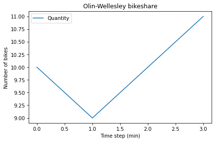
_images/4f14cd8acc6e6a540637a5c77c8b75d12cc706e7f83a9f0ba4fa690b379f2647.png

The result should be a plot with time on the \(x\)-axis and the number of bikes on the \(y\)-axis. Since we only ran three time steps, it might not be very interesting.

Summary#

This chapter introduces the tools we need to run simulations, record the results, and plot them.

We used a State object to represent the state of the system. Then we used the flip function and an if statement to simulate a single time step. We used a for loop to simulate a series of steps, and a TimeSeries to record the results. Finally, we used plot and decorate to plot the results.

In the next chapter, we will extend this simulation to make it a little more realistic.

Exercises#

Before you go on, you might want to work on the following exercises.

Exercise 1#

What happens if you spell the name of a state variable wrong? Edit the following cell, change the spelling of wellesley, and run it.

The error message uses the word attribute, which is another name for what we are calling a state variable.

bikeshare = State(olin=10, wellesley=2)

bikeshare.wellesley

Exercise 2#

Make a State object with a third state variable, called downtown, with initial value 0, and display the state of the system.

Show code cell content Hide code cell content

# Solution

bikeshare = State(olin=10, wellesley=2, downtown=0)
show(bikeshare)

	state
olin	10
wellesley	2
downtown	0

Exercise 3#

Wrap the code in the chapter in a function named run_simulation that takes three parameters, named p1, p2, and num_steps.

It should:

Create a TimeSeries object to hold the results.
Use a for loop to run step the number of times specified by num_steps, passing along the specified values of p1 and p2.
After each step, it should save the number of bikes at Olin in the TimeSeries.
After the for loop, it should plot the results and
Decorate the axes.

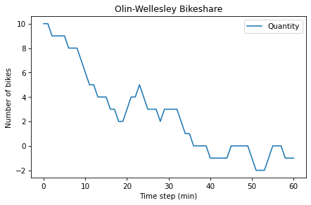
To test your function:

Create a State object with the initial state of the system.
Call run_simulation with parameters p1=0.3, p2=0.2, and num_steps=60.

Under the Hood#

This section contains additional information about the functions we’ve used and pointers to their documentation.

You don’t need to know anything in this section, so if you are already feeling overwhelmed, you might want to skip it. But if you are curious, read on.

State and TimeSeries objects are based on the Series object defined by the Pandas library. The documentation is at https://pandas.pydata.org/pandas-docs/stable/reference/api/pandas.Series.html.

Series objects provide their own plot function, which is why we call it like this:

results.plot()

Instead of like this:

plot(results)

You can read the documentation of Series.plot at https://pandas.pydata.org/pandas-docs/stable/reference/api/pandas.Series.plot.html.

decorate is based on Matplotlib, which is a widely used plotting library for Python. Matplotlib provides separate functions for title, xlabel, and ylabel. decorate makes them a little easier to use. For the list of keyword arguments you can pass to decorate, see https://matplotlib.org/3.2.2/api/axes_api.html?highlight=axes#module-matplotlib.axes.

The flip function uses NumPy’s random function to generate a random number between 0 and 1, then returns True or False with the given probability.

You can get the source code for flip (or any other function) by running the following cell.

source_code(flip)

def flip(p=0.5):
    """Flips a coin with the given probability.

    p: float 0-1

    returns: boolean (True or False)
    """
    return np.random.random() < p