Cooling Coffee

Cooling Coffee#

This chapter is available as a Jupyter notebook where you can read the text, run the code, and work on the exercises. Click here to access the notebooks: https://allendowney.github.io/ModSimPy/.

So far the systems we have studied have been physical in the sense that they exist in the world, but they have not been physics in the sense of what physics classes are usually about. In the next few chapters, we’ll do some physics, starting with thermal systems, that is, systems where the temperature of objects changes as heat transfers from one to another.

The Coffee Cooling Problem#

The coffee cooling problem was discussed by Jearl Walker in “The Amateur Scientist”, Scientific American, Volume 237, Issue 5, November 1977. Since then it has become a standard example of modeling and simulation.

Here is my version of the problem:

Suppose I stop on the way to work to pick up a cup of coffee and a small container of milk. Assuming that I want the coffee to be as hot as possible when I arrive at work, should I add the milk at the coffee shop, wait until I get to work, or add the milk at some point in between?

To help answer this question, I made a trial run with the milk and coffee in separate containers and took some measurements (not really):

When served, the temperature of the coffee is 90 °C. The volume is 300 mL.
The milk is at an initial temperature of 5 °C, and I take about 50 mL.
The ambient temperature in my car is 22 °C.
The coffee is served in a well insulated cup. When I arrive at work after 30 minutes, the temperature of the coffee has fallen to 70 °C.
The milk container is not as well insulated. After 15 minutes, it warms up to 20 °C, nearly the ambient temperature.

To use this data and answer the question, we have to know something about temperature and heat, and we have to make some modeling decisions.

Temperature and Heat#

To understand how coffee cools (and milk warms), we need a model of temperature and heat. Temperature is a property of an object or a system; in SI units it is measured in degrees Celsius (°C). Temperature quantifies how hot or cold the object is, which is related to the average velocity of the particles that make it up.

When particles in a hot object contact particles in a cold object, the hot object gets cooler and the cold object gets warmer as energy is transferred from one to the other. The transferred energy is called heat; in SI units it is measured in joules (J).

Heat is related to temperature by the following equation (see http://modsimpy.com/thermass):

\[Q = C~\Delta T\]

where \(Q\) is the amount of heat transferred to an object, \(\Delta T\) is the resulting change in temperature, and \(C\) is the object’s thermal mass, which is a property of the object that determines how much energy it takes to heat or cool it. In SI units, thermal mass is measured in joules per degree Celsius (J/°C).

For objects made primarily from one material, thermal mass can be computed like this:

\[C = m c_p\]

where \(m\) is the mass of the object and \(c_p\) is the specific heat capacity of the material, which is the amount of thermal mass per gram (see http://modsimpy.com/specheat).

We can use these equations to estimate the thermal mass of a cup of coffee. The specific heat capacity of coffee is probably close to that of water, which is 4.2 J/g/°C. Assuming that the density of coffee is close to that of water, which is 1 g/mL, the mass of 300 mL of coffee is 300 g, and the thermal mass is 1260 J/°C.

So when a cup of coffee cools from 90 °C to 70 °C, the change in temperature, \(\Delta T\) is 20 °C, which means that 25 200 J of heat energy was transferred from the cup and the coffee to the surrounding environment (the cup holder and air in my car).

To give you a sense of how much energy that is, if you were able to harness all of that heat to do work (which you cannot), you could use it to lift a cup of coffee from sea level to 8571 m, just shy of the height of Mount Everest, 8848 m.

Heat Transfer#

In a situation like the coffee cooling problem, there are three ways heat transfers from one object to another (see http://modsimpy.com/transfer):

Conduction: When objects at different temperatures come into contact, the faster-moving particles of the higher-temperature object transfer kinetic energy to the slower-moving particles of the lower-temperature object.
Convection: When particles in a gas or liquid flow from place to place, they carry heat energy with them. Fluid flows can be caused by external action, like stirring, or by internal differences in temperature. For example, you might have heard that hot air rises, which is a form of “natural convection”.
Radiation: As the particles in an object move due to thermal energy, they emit electromagnetic radiation. The energy carried by this radiation depends on the object’s temperature and surface properties (see http://modsimpy.com/thermrad).

For objects like coffee in a car, the effect of radiation is much smaller than the effects of conduction and convection, so we will ignore it.

Convection can be a complex topic, since it often depends on details of fluid flow in three dimensions. But for this problem we will be able to get away with a simple model called “Newton’s law of cooling”.

Newton’s Law of Cooling#

Newton’s law of cooling asserts that the temperature rate of change for an object is proportional to the difference in temperature between the object and the surrounding environment:

\[\frac{dT}{dt} = -r (T - T_{env})\]

where \(t\) is time, \(T\) is the temperature of the object, \(T_{env}\) is the temperature of the environment, and \(r\) is a constant that characterizes how quickly heat is transferred between the object and the environment.

Newton’s so-called “law ” is really a model: it is a good approximation in some conditions and less good in others.

For example, if the primary mechanism of heat transfer is conduction, Newton’s law is “true”, which is to say that \(r\) is constant over a wide range of temperatures. And sometimes we can estimate \(r\) based on the material properties and shape of the object.

When convection contributes a non-negligible fraction of heat transfer, \(r\) depends on temperature, but Newton’s law is often accurate enough, at least over a narrow range of temperatures. In this case \(r\) usually has to be estimated experimentally, since it depends on details of surface shape, air flow, evaporation, etc.

When radiation makes up a substantial part of heat transfer, Newton’s law is not a good model at all. This is the case for objects in space or in a vacuum, and for objects at high temperatures (more than a few hundred degrees Celsius, say).

However, for a situation like the coffee cooling problem, we expect Newton’s model to be quite good.

With that, we have just one more modeling decision to make: whether to treat the coffee and the cup as separate objects or a single object. If the cup is made of paper, it has less mass than the coffee, and the specific heat capacity of paper is lower, too. In that case, it would be reasonable to treat the cup and coffee as a single object. For a cup with substantial thermal mass, like a ceramic mug, we might consider a model that computes the temperature of coffee and cup separately.

Implementing Newtonian Cooling#

To get started, we’ll focus on the coffee. Then, as an exercise, you can simulate the milk. In the next chapter, we’ll put them together, literally.

Here’s a function that takes the parameters of the system and makes a System object:

def make_system(T_init, volume, r, t_end):
    return System(T_init=T_init,
                  T_final=T_init,
                  volume=volume,
                  r=r,
                  t_end=t_end,
                  T_env=22,
                  t_0=0,
                  dt=1)

In addition to the parameters, make_system sets the temperature of the environment, T_env, the initial time stamp, t_0, and the time step, dt, which we will use to simulate the cooling process. Here’s a System object that represents the coffee.

coffee = make_system(T_init=90, volume=300, r=0.01, t_end=30)

The values of T_init, volume, and t_end come from the statement of the problem. I chose the value of r arbitrarily for now; we will see how to estimate it soon.

Strictly speaking, Newton’s law is a differential equation, but over a short period of time we can approximate it with a difference equation:

\[\Delta T = -r (T - T_{env}) dt\]

where \(dt\) is the time step and \(\Delta T\) is the change in temperature during that time step.

Note: I use \(\Delta T\) to denote a change in temperature over time, but in the context of heat transfer, you might also see \(\Delta T\) used to denote the difference in temperature between an object and its environment, \(T - T_{env}\). To minimize confusion, I avoid this second use.

The following function takes the current time t, the current temperature, T, and a System object, and computes the change in temperature during a time step:

def change_func(t, T, system):
    r, T_env, dt = system.r, system.T_env, system.dt    
    return -r * (T - T_env) * dt

We can test it with the initial temperature of the coffee, like this:

change_func(0, coffee.T_init, coffee)

-0.68

With dt=1 minute, the temperature drops by about 0.7 °C, at least for this value of r.

Now here’s a version of run_simulation that simulates a series of time steps from t_0 to t_end:

def run_simulation(system, change_func):
    t_array = linrange(system.t_0, system.t_end, system.dt)
    n = len(t_array)
    
    series = TimeSeries(index=t_array)
    series.iloc[0] = system.T_init
    
    for i in range(n-1):
        t = t_array[i]
        T = series.iloc[i]
        series.iloc[i+1] = T + change_func(t, T, system)
    
    system.T_final = series.iloc[-1]
    return series

There are two things here that are different from previous versions of run_simulation.

First, we use linrange to make an array of values from t_0 to t_end with time step dt. linrange is similar to linspace; they both take a start value and an end value and return an array of equally spaced values. The difference is the third argument: linspace takes an integer that indicates the number of points in the range; linrange takes a step size that indicates the interval between values. When we make the TimeSeries, we use the keyword argument index to indicate that the index of the TimeSeries is the array of time stamps, t_array.

Second, this version of run_simulation uses iloc rather than loc to specify the rows in the TimeSeries. Here’s the difference:

With loc, the label in brackets can be any kind of value, with any start, end, and time step. For example, in the world population model, the labels are years starting in 1960 and ending in 2016.
With iloc, the label in brackets is always an integer starting at 0. So we can always get the first element with iloc[0] and the last element with iloc[-1], regardless of what the labels are.

In this version of run_simulation, the loop variable is an integer, i, that goes from 0 to n-1, including 0 but not including n-1. So the first time through the loop, i is 0 and the value we add to the TimeSeries has index 1. The last time through the loop, i is n-2 and the value we add has index n-1.

We can run the simulation like this:

results = run_simulation(coffee, change_func)

The result is a TimeSeries with one row per time step. Here are the first few rows:

show(results.head())

	Quantity
Time
0.0	90.000000
1.0	89.320000
2.0	88.646800
3.0	87.980332
4.0	87.320529

And the last few rows:

show(results.tail())

	Quantity
Time
26.0	74.362934
27.0	73.839305
28.0	73.320912
29.0	72.807702
30.0	72.299625

With t_0=0, t_end=30, and dt=1, the time stamps go from 0.0 to 30.0.

Here’s what the TimeSeries looks like.

results.plot(label='coffee')

decorate(xlabel='Time (min)',
         ylabel='Temperature (C)',
         title='Coffee Cooling')

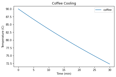
_images/71f824fe8df44e3a145492aa879121ae3c730de336d50a6bed515912c44b34e7.png

The temperature after 30 minutes is 72.3 °C, which is a little higher than the measurement we’re trying to match, which is 70 °C.

coffee.T_final

72.2996253904031

To find the value of r where the final temperature is precisely 70 °C, we could proceed by trial and error, but it is more efficient to use a root-finding algorithm.

Finding Roots#

The ModSim library provides a function called root_scalar that finds the roots of non-linear equations. As an example, suppose you want to find the roots of the polynomial

\[f(x) = (x - 1)(x - 2)(x - 3)\]

A root is a value of \(x\) that makes \(f(x)=0\). Because of the way I wrote this polynomial, we can see that if \(x=1\), the first factor is 0; if \(x=2\), the second factor is 0; and if \(x=3\), the third factor is 0, so those are the roots.

I’ll use this example to demonstrate root_scalar. First, we have to write a function that evaluates \(f\):

def func(x):
    return (x-1) * (x-2) * (x-3)

Now we call root_scalar like this:

res = root_scalar(func, bracket=[1.5, 2.5])
res

      converged: True
           flag: 'converged'
 function_calls: 3
     iterations: 2
           root: 2.0

The first argument is the function whose roots we want. The second argument is an interval that contains or brackets a root. The result is an object that contains several variables, including the Boolean value converged, which is True if the search converged successfully on a root, and root, which is the root that was found.

res.root

2.0

If we provide a different interval, we find a different root.

res = root_scalar(func, bracket=[2.5, 3.5])
res.root

2.9999771663211003

If the interval doesn’t contain a root, you’ll get a ValueError and a message like f(a) and f(b) must have different signs.

Now we can use root_scalar to estimate r.

Estimating r#

What we want is the value of r that yields a final temperature of 70 °C. To use root_scalar, we need a function that takes r as a parameter and returns the difference between the final temperature and the goal:

def error_func(r, system):
    system.r = r
    results = run_simulation(system, change_func)
    return system.T_final - 70

This is called an error function because it returns the difference between what we got and what we wanted, that is, the error. With the right value of r, the error is 0.

We can test error_func like this, using the initial guess r=0.01:

coffee = make_system(T_init=90, volume=300, r=0.01, t_end=30)
error_func(0.01, coffee)

2.2996253904030937

The result is an error of 2.3 °C, which means the final temperature with r=0.01 is too high.

error_func(0.02, coffee)

-10.907066281994297

With r=0.02, the error is about -11°C, which means that the final temperature is too low. So we know that the correct value must be in between.

Now we can call root_scalar like this:

res = root_scalar(error_func, coffee, bracket=[0.01, 0.02])
res

      converged: True
           flag: 'converged'
 function_calls: 6
     iterations: 5
           root: 0.011543084190599507

The first argument is the error function. The second argument is the System object, which root_scalar passes as an argument to error_func. The third argument is an interval that brackets the root.

Here’s the root we found.

r_coffee = res.root
r_coffee

0.011543084190599507

In this example, r_coffee turns out to be about 0.0115, in units of min\(^{-1}\) (inverse minutes). We can confirm that this value is correct by setting r to the root we found and running the simulation.

coffee.r = res.root
run_simulation(coffee, change_func)
coffee.T_final

70.00000057308064

The final temperature is very close to 70 °C.

Summary#

This chapter presents the basics of heat, temperature, and Newton’s law of cooling, which is a model that is accurate when most heat transfer is by conduction and convection, not radiation.

To simulate a hot cup of coffee, we wrote Newton’s law as a difference equation, then wrote a version of run_simulation that implements it. Then we used root_scalar to find the value of r that matches the measurement from my hypothetical experiment.

All that is the first step toward solving the coffee cooling problem I posed at the beginning of the chapter. As an exercise, you’ll do the next step, which is simulating the milk. In the next chapter, we’ll model the mixing process and finish off the problem.

Exercises#

This chapter is available as a Jupyter notebook where you can read the text, run the code, and work on the exercises. You can access the notebooks at https://allendowney.github.io/ModSimPy/.

Exercise 1#

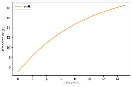
Simulate the temperature of 50 mL of milk with a starting temperature of 5 °C, in a vessel with r=0.1, for 15 minutes, and plot the results. Use make_system to make a System object that represents the milk, and use run_simulation to simulate it. By trial and error, find a value for r that makes the final temperature close to 20 °C.

Exercise 2#

Write an error function that simulates the temperature of the milk and returns the difference between the final temperature and 20 °C. Use it to estimate the value of r for the milk.