Testing Order of Growth
Contents
Testing Order of Growth#
Click here to run this chapter on Colab
Analysis of algorithms makes it possible to predict how run time will grow as the size of a problem increases. But this kind of analysis ignores leading coefficients and non-leading terms. So the behavior for small and medium problems might not be what the analysis predicts.
To see how run time really behaves for a range of problem sizes, we can run the algorithm and measure.
To do the measurement, we’ll use the times function from the os module.
import os

def etime():
    """Measures user and system time this process has used.

    Returns the sum of user and system time."""
    user, sys, chuser, chsys, real = os.times()
    return user+sys
start = etime()
t = [x**2 for x in range(10000)]
end = etime()
end - start
0.0
Exercise: Use etime to measure the computation time used by sleep.
from time import sleep

sleep(1)
def time_func(func, n):
    """Run a function and return the elapsed time.

    func: function
    n: problem size, passed as an argument to func

    returns: user+sys time in seconds
    """
    start = etime()
    func(n)
    end = etime()
    elapsed = end - start
    return elapsed
One of the things that makes timing tricky is that many operations are too fast to measure accurately.
%timeit handles this by running enough times get a precise estimate, even for things that run very fast.
We’ll handle it by running over a wide range of problem sizes, hoping to find sizes that run long enough to measure, but not more than a few seconds.
The following function takes a size, n, creates an empty list, and calls list.append n times.
def list_append(n):
    t = []
    [t.append(x) for x in range(n)]
timeit can time this function accurately.
%timeit list_append(10000)
427 µs ± 6.66 µs per loop (mean ± std. dev. of 7 runs, 1000 loops each)
But our time_func is not that smart.
time_func(list_append, 10000)
0.0
Exercise: Increase the number of iterations until the run time is measureable.
List append#
The following function gradually increases n and records the total time.
def run_timing_test(func, max_time=1):
    """Tests the given function with a range of values for n.

    func: function object

    returns: list of ns and a list of run times.
    """
    ns = []
    ts = []
    for i in range(10, 28):
        n = 2**i
        t = time_func(func, n)
        print(n, t)
        if t > 0:
            ns.append(n)
            ts.append(t)
        if t > max_time:
            break

    return ns, ts
ns, ts = run_timing_test(list_append)
1024 0.0
2048 0.0
4096 0.0
8192 0.0
16384 0.009999999999999787
32768 0.0
65536 0.0
131072 0.020000000000000462
262144 0.019999999999999574
524288 0.02999999999999936
1048576 0.08000000000000096
2097152 0.15999999999999925
4194304 0.27000000000000046
8388608 0.5700000000000003
16777216 1.0399999999999991
import matplotlib.pyplot as plt

plt.plot(ns, ts, 'o-')
plt.xlabel('Problem size (n)')
plt.ylabel('Runtime (seconds)');
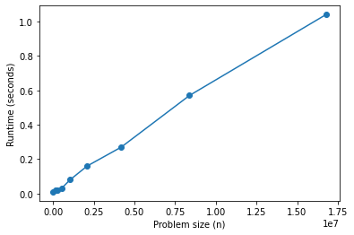
This one looks pretty linear, but it won’t always be so clear. It will help to plot a straight line that goes through the last data point.
def fit(ns, ts, exp=1.0, index=-1):
    """Fits a curve with the given exponent.

    ns: sequence of problem sizes
    ts: sequence of times
    exp: exponent of the fitted curve
    index: index of the element the fitted line should go through

    returns: sequence of fitted times


    """
    # Use the element with the given index as a reference point,
    # and scale all other points accordingly.
    nref = ns[index]
    tref = ts[index]

    tfit = []
    for n in ns:
        ratio = n / nref
        t = ratio**exp * tref
        tfit.append(t)

    return tfit
ts_fit = fit(ns, ts)
ts_fit
[0.0010156249999999992,
 0.008124999999999993,
 0.016249999999999987,
 0.03249999999999997,
 0.06499999999999995,
 0.1299999999999999,
 0.2599999999999998,
 0.5199999999999996,
 1.0399999999999991]
The following function plots the actual results and the fitted line.
def plot_timing_test(ns, ts, label='', color='C0', exp=1.0, scale='log'):
    """Plots data and a fitted curve.

    ns: sequence of n (problem size)
    ts: sequence of t (run time)
    label: string label for the data curve
    color: string color for the data curve
    exp: exponent (slope) for the fitted curve
    scale: string passed to xscale and yscale
    """
    ts_fit = fit(ns, ts, exp)
    fit_label = 'exp = %d' % exp
    plt.plot(ns, ts_fit, label=fit_label, color='0.7', linestyle='dashed')
    plt.plot(ns, ts, 'o-', label=label, color=color, alpha=0.7)
    plt.xlabel('Problem size (n)')
    plt.ylabel('Runtime (seconds)')
    plt.xscale(scale)
    plt.yscale(scale)
    plt.legend()
plot_timing_test(ns, ts, scale='linear')
plt.title('list append');
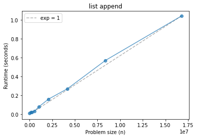
From these results, what can we conclude about the order of growth of list.append?
Before we go on, let’s also look at the results on a log-log scale.
plot_timing_test(ns, ts, scale='log')
plt.title('list append');
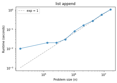
Why might we prefer this scale?
List pop#
Now let’s do the same for list.pop (which pops from the end of the list by default).
Notice that we have to make the list before we pop things from it, so we will have to think about how to interpret the results.
def list_pop(n):
    t = []
    [t.append(x) for x in range(n)]
    [t.pop() for _ in range(n)]

ns, ts = run_timing_test(list_pop)
plot_timing_test(ns, ts, scale='log')
plt.title('list pop');
1024 0.0
2048 0.0
4096 0.0
8192 0.010000000000001563
16384 0.0
32768 0.0
65536 0.009999999999999787
131072 0.009999999999999787
262144 0.03999999999999915
524288 0.05000000000000071
1048576 0.11000000000000121
2097152 0.22999999999999865
4194304 0.4800000000000004
8388608 0.8699999999999992
16777216 1.6900000000000013
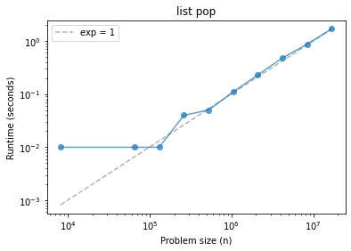
What can we conclude?
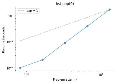
What about pop(0), which pops from the beginning of the list?
Note: You might have to adjust exp to make the fitted line fit.
def list_pop0(n):
    t = []
    [t.append(x) for x in range(n)]
    [t.pop(0) for _ in range(n)]

ns, ts = run_timing_test(list_pop0)
plot_timing_test(ns, ts, scale='log', exp=1)
plt.title('list pop(0)');
1024 0.0
2048 0.0
4096 0.0
8192 0.010000000000001563
16384 0.019999999999999574
32768 0.08999999999999986
65536 0.39000000000000057
131072 1.7199999999999989
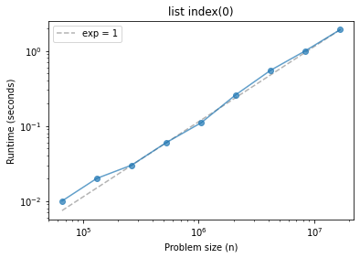
Searching a list#
list.index searches a list and returns the index of the first element that matches the target.
What do we expect if we always search for the first element?
def list_index0(n):
    t = []
    [t.append(x) for x in range(n)]
    [t.index(0) for _ in range(n)]

ns, ts = run_timing_test(list_index0)

plot_timing_test(ns, ts, scale='log', exp=1)
plt.title('list index(0)');
1024 0.0
2048 0.0
4096 0.0
8192 0.0
16384 0.0
32768 0.0
65536 0.009999999999999787
131072 0.019999999999999574
262144 0.030000000000001137
524288 0.05999999999999872
1048576 0.10999999999999943
2097152 0.26000000000000156
4194304 0.5500000000000007
8388608 1.0
16777216 1.9100000000000001
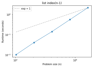
What if we always search for the last element?
def list_index_n(n):
    t = []
    [t.append(x) for x in range(n)]
    [t.index(n-1) for _ in range(n)]

ns, ts = run_timing_test(list_index_n)

plot_timing_test(ns, ts, scale='log', exp=1)
plt.title('list index(n-1)');
1024 0.00999999999999801
2048 0.03999999999999915
4096 0.14000000000000057
8192 0.5499999999999972
16384 2.1400000000000006
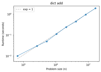
Dictionary add#
def dict_add(n):
    d = {}
    [d.setdefault(x, x) for x in range(n)]

ns, ts = run_timing_test(dict_add)

plot_timing_test(ns, ts, scale='log', exp=1)
plt.title('dict add');
1024 0.0
2048 0.0
4096 0.0
8192 0.0
16384 0.0
32768 0.0
65536 0.00999999999999801
131072 0.0
262144 0.030000000000001137
524288 0.04999999999999716
1048576 0.11000000000000298
2097152 0.23999999999999844
4194304 0.4400000000000013
8388608 0.9400000000000013
16777216 1.8699999999999974
Dictionary lookup#
def dict_lookup(n):
    d = {}
    [d.setdefault(x, x) for x in range(n)]
    [d[x] for x in range(n)]

ns, ts = run_timing_test(dict_lookup)

plot_timing_test(ns, ts, scale='log', exp=1)
plt.title('dict lookup');
1024 0.0
2048 0.0
4096 0.0
8192 0.0
16384 0.0
32768 0.00999999999999801
65536 0.010000000000005116
131072 0.01999999999999602
262144 0.05000000000000071
524288 0.06999999999999673
1048576 0.1600000000000037
2097152 0.33999999999999986
4194304 0.6600000000000001
8388608 1.3900000000000006
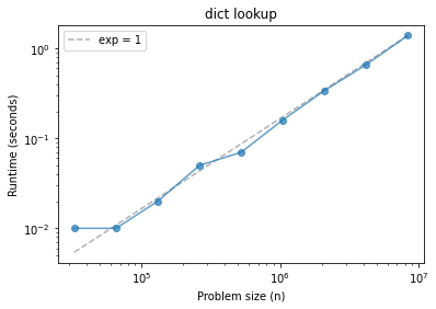
This characteristic of dictionaries is the foundation of a lot of efficient algorithms!