FFT#

Click here to run this chapter on Colab

from os.path import basename, exists

def download(url):
    filename = basename(url)
    if not exists(filename):
        from urllib.request import urlretrieve
        local, _ = urlretrieve(url, filename)
        print('Downloaded ' + local)
    
download('https://github.com/AllenDowney/DSIRP/raw/main/timing.py')

from timing import run_timing_test, plot_timing_test

Discrete Fourier Transform#

According to our friends at Wikipedia:

The discrete Fourier transform transforms a sequence of $N$ complex numbers $x = x_{0}, x_{1}, \dots, x_{N - 1}$ into another sequence of complex numbers, $X = X_{0}, X_{1}, \dots, X_{N - 1},$ which is defined by $ $X_{k} = \sum_{n = 0}^{N} x_{n} \cdot e^{- i 2 π k n / N}$ $

Notice:

$X$ and $x$ are the same length, $N$ .
$n$ is the index that specifies an element of $x$ , and
$k$ is the index that specifies an element of $X$ .

Let’s start with a small example and use Numpy’s implementation of FFT to compute the DFT.

x = [1, 0, 0, 0]

import numpy as np

np.fft.fft(x)

array([1.+0.j, 1.+0.j, 1.+0.j, 1.+0.j])

Now we know what the answer is, let’s compute it ourselves.

Here’s the expression that computes one element of $X$ .

pi = np.pi
exp = np.exp
N = len(x)
k = 0

sum(x[n] * exp(-2j * pi * k * n / N) for n in range(N))

(1+0j)

Wrapping this code in a function makes the roles of k and n clearer:

k is the parameter that specifies which element of the DFT to compute, and
n is the loop variable we use to compute the summation.

def dft_k(x, k):
    N = len(x)
    return sum(x[n] * exp(-2j * pi * k * n / N) for n in range(N))

dft_k(x, k=1)

(1+0j)

Usually we compute $X$ all at once, so we can wrap dft_k in another function:

def dft(x):
    N = len(x)
    X = [dft_k(x, k) for k in range(N)]
    return X

dft(x)

[(1+0j), (1+0j), (1+0j), (1+0j)]

And that’s what we got from Numpy.

Timing DFT#

Let’s see what the performance of dft looks like.

def test_dft(N):
    x = np.random.normal(size=N)
    X = dft(x)

%time test_dft(512)

CPU times: user 772 ms, sys: 44 µs, total: 772 ms
Wall time: 772 ms

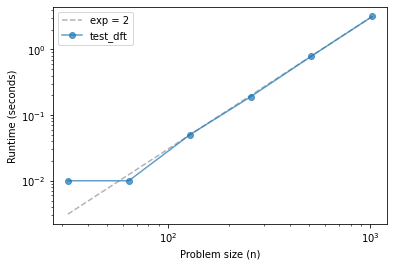
ns, ts = run_timing_test(test_dft, start_at=5)
plot_timing_test(ns, ts, 'test_dft', exp=2)

32 0.010000000000000231
64 0.009999999999999787
128 0.050000000000000266
256 0.18999999999999995
512 0.79
1024 3.1799999999999993

Implementing FFT#

The key to the FFT algorithm is the Danielson-Lanczos lemma, which says

$X_{k} = E_{k} + e^{- i 2 π n / N} O_{k}$

Where

$E$ is the FFT of the even elements of $x$ , and
$O$ is the DFT of the odd elements of $x$ .

Before we can translate this expression into code, we have to deal with a gotcha.

Remember that, if the length of $x$ is $N$ , the length of $X$ is also $N$ .

If we select the even elements of $x$ , the result is a sequence with length $N / 2$ , which means that the length of $E$ is $N / 2$ . And the same for $O$ .

But if $k$ goes from $0$ up to $N - 1$ , what do we do when it exceeds $N / 2 - 1$ ?

Fortunately, the DFT repeats itself so, $X_{N}$ is the same as $X_{0}$ . That means we can extend $E$ and $O$ to be the same length as $X$ just by repeating them. And we can do that with the Numpy function tile.

So, here’s a version of merge based on the D-L lemma.

def merge(E, O):
    N = len(E) * 2
    ns = np.arange(N)
    W = np.exp(-2j * pi * ns / N)
    return np.tile(E, 2) + W * np.tile(O, 2)

Exercise: As a first step toward implementing FFT, write a non-recursive function called fft_norec that takes a sequence called x and

Divides x into even and odd elements,
Uses dft to compute E and O, and
Uses merge to compute X.

fft_norec(x)

array([1.+0.j, 1.+0.j, 1.+0.j, 1.+0.j])

Let’s see what the performance looks like.

def test_fft_norec(N):
    x = np.random.normal(size=N)
    spectrum = fft_norec(x)

%time test_fft_norec(512)

CPU times: user 384 ms, sys: 3.38 ms, total: 388 ms
Wall time: 387 ms

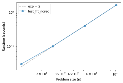
ns, ts = run_timing_test(test_fft_norec, start_at=5)
plot_timing_test(ns, ts, 'test_fft_norec', exp=2)

32 0.0
64 0.0
128 0.030000000000001137
256 0.09999999999999964
512 0.3899999999999988
1024 1.5899999999999999

Exercise: Starting with fft_norec, write a function called fft_rec that’s fully recursive; that is, instead of using dft to compute the DFTs of the halves, it should use fft_rec.

You will need a base case to avoid an infinite recursion. You have two options:

The DFT of an array with length 1 is the array itself.
If the parameter, x, is smaller than some threshold length, you could use DFT.

Use test_fft_rec, below, to check the performance of your function.

fft_rec(x)

array([1.+0.j, 1.+0.j, 1.+0.j, 1.+0.j])

def test_fft_rec(N):
    x = np.random.normal(size=N)
    spectrum = fft_rec(x)

%time test_fft_rec(512)

CPU times: user 8.36 ms, sys: 42 µs, total: 8.4 ms
Wall time: 7.92 ms

ns, ts = run_timing_test(test_fft_rec)
plot_timing_test(ns, ts, 'test_fft_rec', exp=1)

1024 0.019999999999999574
2048 0.030000000000001137
4096 0.049999999999998934
8192 0.11000000000000121
16384 0.22999999999999865
32768 0.45000000000000107
65536 0.9000000000000004
131072 1.83

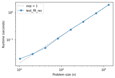
If things go according to plan, your FFT implementation should be faster than dft and fft_norec, and over a range of problem sizes, it might be indistinguishable from linear.

Data Structures and Information Retrieval in Python

License: Creative Commons Attribution-NonCommercial-ShareAlike 4.0 International

Data Structures and Information Retrieval in Python

FFT

Contents

FFT#

Discrete Fourier Transform#

Timing DFT#

Implementing FFT#