Analysis of Algorithms
Contents
Analysis of Algorithms#
Click here to run this chapter on Colab
Analysis of algorithms is a branch of computer science that studies the performance of algorithms, especially their run time and space requirements. See http://en.wikipedia.org/wiki/Analysis_of_algorithms.
The practical goal of algorithm analysis is to predict the performance of different algorithms in order to guide design decisions.
During the 2008 United States Presidential Campaign, candidate Barack Obama was asked to perform an impromptu analysis when he visited Google. Chief executive Eric Schmidt jokingly asked him for “the most efficient way to sort a million 32-bit integers.” Obama had apparently been tipped off, because he quickly replied, “I think the bubble sort would be the wrong way to go.” See http://www.youtube.com/watch?v=k4RRi_ntQc8.
This is true: bubble sort is conceptually simple but slow for large datasets. The answer Schmidt was probably looking for is “radix sort” (http://en.wikipedia.org/wiki/Radix_sort).
But if you get a question like this in an interview, I think a better answer is, “The fastest way to sort a million integers is to use whatever sort function is provided by the language I’m using. Its performance is good enough for the vast majority of applications, but if it turned out that my application was too slow, I would use a profiler to see where the time was being spent. If it looked like a faster sort algorithm would have a significant effect on performance, then I would look around for a good implementation of radix sort.”
The goal of algorithm analysis is to make meaningful comparisons between algorithms, but there are some problems:
The relative performance of the algorithms might depend on characteristics of the hardware, so one algorithm might be faster on Machine A, another on Machine B. The usual solution to this problem is to specify a machine model and analyze the number of steps, or operations, an algorithm requires under a given model.
Relative performance might depend on the details of the dataset. For example, some sorting algorithms run faster if the data are already partially sorted; other algorithms run slower in this case. A common way to avoid this problem is to analyze the worst case scenario. It is sometimes useful to analyze average case performance, but that’s usually harder, and it might not be obvious what set of cases to average over.
Relative performance also depends on the size of the problem. A sorting algorithm that is fast for small lists might be slow for long lists. The usual solution to this problem is to express run time (or number of operations) as a function of problem size, and group functions into categories depending on how quickly they grow as problem size increases.
The good thing about this kind of comparison is that it lends itself to simple classification of algorithms. For example, if I know that the run time of Algorithm A tends to be proportional to the size of the input, \(n\), and Algorithm B tends to be proportional to \(n^2\), then I expect A to be faster than B, at least for large values of \(n\).
This kind of analysis comes with some caveats, but we’ll get to that later.
Order of growth#
Suppose you have analyzed two algorithms and expressed their run times in terms of the size of the input: Algorithm A takes \(100n+1\) steps to solve a problem with size \(n\); Algorithm B takes \(n^2 + n + 1\) steps.
The following table shows the run time of these algorithms for different problem sizes:
import numpy as np
import pandas as pd

n = np.array([10, 100, 1000, 10000])
table = pd.DataFrame(index=n)
table['Algorithm A'] = 100 * n + 1
table['Algorithm B'] = n**2 + n + 1
table['Ratio (B/A)'] = table['Algorithm B'] / table['Algorithm A']
table
| Algorithm A | Algorithm B | Ratio (B/A) | |
|---|---|---|---|
| 10 | 1001 | 111 | 0.110889 |
| 100 | 10001 | 10101 | 1.009999 |
| 1000 | 100001 | 1001001 | 10.009910 |
| 10000 | 1000001 | 100010001 | 100.009901 |
At \(n=10\), Algorithm A looks pretty bad; it takes almost 10 times longer than Algorithm B. But for \(n=100\) they are about the same, and for larger values A is much better.
The fundamental reason is that for large values of \(n\), any function that contains an \(n^2\) term will grow faster than a function whose leading term is \(n\). The leading term is the term with the highest exponent.
For Algorithm A, the leading term has a large coefficient, 100, which is why B does better than A for small \(n\). But regardless of the coefficients, there will always be some value of \(n\) where \(a n^2 > b n\), for any values of \(a\) and \(b\).
The same argument applies to the non-leading terms. Suppose the run time of Algorithm C is \(n+1000000\); it would still be better than Algorithm B for sufficiently large \(n\).
import numpy as np
import pandas as pd

n = np.array([10, 100, 1000, 10000])
table = pd.DataFrame(index=n)
table['Algorithm C'] = n + 1000000
table['Algorithm B'] = n**2 + n + 1
table['Ratio (C/B)'] = table['Algorithm B'] / table['Algorithm C']
table
| Algorithm C | Algorithm B | Ratio (C/B) | |
|---|---|---|---|
| 10 | 1000010 | 111 | 0.000111 |
| 100 | 1000100 | 10101 | 0.010100 |
| 1000 | 1001000 | 1001001 | 1.000001 |
| 10000 | 1010000 | 100010001 | 99.019803 |
In general, we expect an algorithm with a smaller leading term to be a better algorithm for large problems, but for smaller problems, there may be a crossover point where another algorithm is better.
The following figure shows the run times (in arbitrary units) for the three algorithms over a range of problems sizes. For small problem sizes, Algorithm B is the fastest, but for large problems sizes, it is the worst. In the figure, we can see where the crossover points are.
import matplotlib.pyplot as plt

ns = np.arange(10, 1500)
ys = 100 * ns + 1
plt.plot(ns, ys, label='Algorithm A')

ys = ns**2 + ns + 1
plt.plot(ns, ys, label='Algorithm B')

ys = ns + 1_000_000
plt.plot(ns, ys, label='Algorithm C')

plt.yscale('log')
plt.xlabel('Problem size (n)')
plt.ylabel('Run time')
plt.legend();
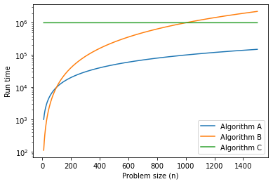
The location of these crossover points depends on the details of the algorithms, the inputs, and the hardware, so it is usually ignored for purposes of algorithmic analysis. But that doesn’t mean you can forget about it.
Big O notation#
If two algorithms have the same leading order term, it is hard to say which is better; again, the answer depends on the details. So for algorithmic analysis, functions with the same leading term are considered equivalent, even if they have different coefficients.
An order of growth is a set of functions whose growth behavior is considered equivalent. For example, \(2n\), \(100n\) and \(n+1\) belong to the same order of growth, which is written \(O(n)\) in Big-O notation and often called linear because every function in the set grows linearly with \(n\).
All functions with the leading term \(n^2\) belong to \(O(n^2)\); they are called quadratic.
The following table shows some of the orders of growth that appear most commonly in algorithmic analysis, in increasing order of badness.
Order of growth |
Name |
|---|---|
\(O(1)\) |
constant |
\(O(\log_b n)\) |
logarithmic (for any \(b\)) |
\(O(n)\) |
linear |
\(O(n \log_b n)\) |
linearithmic |
\(O(n^2)\) |
quadratic |
\(O(n^3)\) |
cubic |
\(O(c^n)\) |
exponential (for any \(c\)) |
For the logarithmic terms, the base of the logarithm doesn’t matter; changing bases is the equivalent of multiplying by a constant, which doesn’t change the order of growth. Similarly, all exponential functions belong to the same order of growth regardless of the base of the exponent. Exponential functions grow very quickly, so exponential algorithms are only useful for small problems.
Exercise#
Read the Wikipedia page on Big-O notation at http://en.wikipedia.org/wiki/Big_O_notation and answer the following questions:
What is the order of growth of \(n^3 + n^2\)? What about \(1000000 n^3 + n^2\)? What about \(n^3 + 1000000 n^2\)?
What is the order of growth of \((n^2 + n) \cdot (n + 1)\)? Before you start multiplying, remember that you only need the leading term.
If \(f\) is in \(O(g)\), for some unspecified function \(g\), what can we say about \(af+b\), where \(a\) and \(b\) are constants?
If \(f_1\) and \(f_2\) are in \(O(g)\), what can we say about \(f_1 + f_2\)?
If \(f_1\) is in \(O(g)\) and \(f_2\) is in \(O(h)\), what can we say about \(f_1 + f_2\)?
If \(f_1\) is in \(O(g)\) and \(f_2\) is in \(O(h)\), what can we say about \(f_1 \cdot f_2\)?
Programmers who care about performance often find this kind of analysis hard to swallow. They have a point: sometimes the coefficients and the non-leading terms make a real difference. Sometimes the details of the hardware, the programming language, and the characteristics of the input make a big difference. And for small problems, order of growth is irrelevant.
But if you keep those caveats in mind, algorithmic analysis is a useful tool. At least for large problems, the “better” algorithm is usually better, and sometimes it is much better. The difference between two algorithms with the same order of growth is usually a constant factor, but the difference between a good algorithm and a bad algorithm is unbounded!
Example: Adding the elements of a list#
In Python, most arithmetic operations are constant time; multiplication usually takes longer than addition and subtraction, and division takes even longer, but these run times don’t depend on the magnitude of the operands. Very large integers are an exception; in that case the run time increases with the number of digits.
A for loop that iterates a list is linear, as long as all of the operations in the body of the loop are constant time. For example, adding up the elements of a list is linear:
def compute_sum(t):
    total = 0
    for x in t:
        total += x
    return total
t = range(10)
compute_sum(t)
45
The built-in function sum is also linear because it does the same thing, but it tends to be faster because it is a more efficient implementation; in the language of algorithmic analysis, it has a smaller leading coefficient.
%timeit compute_sum(t)
303 ns ± 1.26 ns per loop (mean ± std. dev. of 7 runs, 1000000 loops each)
%timeit sum(t)
Example: Sorting#
Python provides a list method, sort, that modifies a list in place, and a function, sorted that makes a new list.
Read the Wikipedia page on sorting algorithms at http://en.wikipedia.org/wiki/Sorting_algorithm and answer the following questions:
What is a “comparison sort?” What is the best worst-case order of growth for a comparison sort? What is the best worst-case order of growth for any sort algorithm?
What is the order of growth of bubble sort, and why does Barack Obama think it is “the wrong way to go?”
What is the order of growth of radix sort? What preconditions do we need to use it?
What is a stable sort and why might it matter in practice?
What is the worst sorting algorithm (that has a name)?
What sort algorithm does the C library use? What sort algorithm does Python use? Are these algorithms stable? You might have to Google around to find these answers.
Many of the non-comparison sorts are linear, so why does Python use an \(O(n \log n)\) comparison sort?
Data Structures and Information Retrieval in Python
Copyright 2021 Allen Downey
License: Creative Commons Attribution-NonCommercial-ShareAlike 4.0 International