Search#

Linear Search#

Suppose you have a list.

t = [5, 1, 2, 4, 2]

And you want to know whether an element appears in the list. You can use the in operator, which returns True or False.

5 in t, 6 in t

(True, False)

If you want to know where in the list it is, you can use index, which returns the index of the element if it appears.

t.index(2)

Or raises a ValueError otherwise.

try:
    t.index(6)
except ValueError as e:
    print(e)

6 is not in list

The following function does the same thing as string.index:

def index(t, target):
    for i, x in enumerate(t):
        if x == target:
            return i
    raise ValueError(f'{target} is not in list')

index(t, 2)

try:
    index(t, 6)
except ValueError as e:
    print(e)

6 is not in list

The runtime of this kind of search is in O(n), where n is the length of the list, because

If the target is not in the list, you have to check every element in the list.
If the target is in a random location, you have to check half the list on average.

As an exception, if you know that the target is within the first k elements, for a value of k that does not depend on n, you can consider this search O(1).

Bisection#

If we know that the elements of the list are in order, we can do better.

The bisect module provides an implementation of a “bisection search”, which works by

Checking the element in the middle of the list. If it’s the target, we’re done.
If the middle element is larger than the target, we search the left half.
If the middle element is smaller than the target, we search the right half.

Here is the documentation of the bisect modle.

To test it, we’ll start with a sorted list.

t.sort()
t

[1, 2, 2, 4, 5]

bisect_left is similar to index

from bisect import bisect_left

bisect_left(t, 1), bisect_left(t, 2), bisect_left(t, 4), bisect_left(t, 5) 

(0, 1, 3, 4)

But with elements that are not in the list, it returns their insertion point, that is, the place where you would put the target to keep the list sorted.

bisect_left(t, 6)

We can use bisect_left to implement index, like this:

from bisect import bisect_left

def index_bisect(a, x):
    """Locate the leftmost value exactly equal to x"""
    i = bisect_left(a, x)
    if i != len(a) and a[i] == x:
        return i
    raise ValueError(f'{x} not in list')

index_bisect(t, 1), index_bisect(t, 2), index_bisect(t, 4), index_bisect(t, 5) 

(0, 1, 3, 4)

try:
    index_bisect(t, 6)
except ValueError as e:
    print(e)

6 not in list

Exercise: Write your own version of bisect_left. You can do it iteratively or recursively.

Each time through the loop, we cut the search region in half, so if we start with n elements, we have n/2 during the next loop, n/4 during the second loop, and so on. When we get to 1 element, we’re done.

See this animation

So how many steps does that take? Thinking about it in reverse, starting with 1, how many times do we have to double it before we get to n? In math notation, the question is

\[2^x = n\]

Where x is the unknown number of steps. Taking the log of both sides, base 2:

\[x = log_2 n\]

In terms of order of growth, bisection search is in O(log n). Notice that we don’t bother to specify the base of the logarithm, because a log in one base is a constant multiple of a log in any other base.

bisect also provides methods to insert elements while maintaining sorted order.

from bisect import insort

insort(t, 3)
t

[1, 2, 2, 3, 4, 5]

However, as the documentation explains, “Keep in mind that the O(log n) search is dominated by the slow O(n) insertion step.”

Binary search tree#

Using a sorted array to support log-time search is a reasonable choice if we don’t have to add or remove elements very often.

But if the number of add/remove operations is similar to the number of searches, the overall performance would be linear.

We can solve that problem with a binary search tree.

To implement a tree, I’ll define a new class that represents a Node. Each node contains data and a reference to two “children” called left and right. (It’s called a binary tree because every node has two children).

class Node:
    def __init__(self, data, left=None, right=None):
        self.data = data
        self.left = left
        self.right = right
        
    def __repr__(self):
        return f'Node({self.data}, {repr(self.left)}, {repr(self.right)})'

Here’s how we can instantiate two nodes.

node3 = Node(3)
node10 = Node(10)

Because Node provides __repr__, we can display a node like this.

node3

Node(3, None, None)

Now we’ll make a parent node that has the first two nodes as children.

node8 = Node(8, node3, node10)
node8

Node(8, Node(3, None, None), Node(10, None, None))

I’ll define another class to represent the tree. The only thing it contains is a reference to the top of the tree, which is confusingly called the root node.

class BSTree:
    def __init__(self, root=None):
        self.root = root
        
    def __repr__(self):
        return f'BSTree({repr(self.root)})'

Here’s tree with a reference to node8, so it implicitly contains node3 and node10 as well.

tree = BSTree(node8)
tree

BSTree(Node(8, Node(3, None, None), Node(10, None, None)))

A binary tree is a binary search tree if for every node (1) the value of the left child is lower and (2) the value of the right child is higher. Let’s assume for now that there are no duplicates.

We can check whether a tree is a BST like this:

def is_bst(tree):
    return is_bst_rec(tree.root)

def is_bst_rec(node):
    if node is None:
        return True
    
    if node.left and node.left.data > node.data:
        return False
    if node.right and node.right.data < node.data:
        return False
    
    return is_bst_rec(node.left) and is_bst_rec(node.right)

is_bst(tree)

True

And let’s see an example where it’s not true.

node5 = Node(5, node10, node3)
node5

Node(5, Node(10, None, None), Node(3, None, None))

tree2 = BSTree(node5)
is_bst(tree2)

False

Draw the Tree#

One of the better functions for drawing trees is part of a package called EoN, for “Epidemics on Networks”, which provides “tools to study the spread of SIS and SIR diseases in networks”.

The function we’ll use is called hierarchy_pos. It takes as a parameter a NetworkX graph that represents a tree, and it returns a dictionary that maps from each node to a position in the Cartesian plane. If we pass this dictionary to nx.draw, it lays the tree out accordingly.

try:
    import EoN
except ImportError:
    !pip install EoN

import networkx as nx

def add_edges(node, G):
    """Make a NetworkX graph that represents the heap."""
    if node is None:
        return
    
    G.add_node(node, label=node.data)
    for child in (node.left, node.right):
        if child:
            G.add_edge(node, child)
            add_edges(child, G)

G = nx.DiGraph()
add_edges(tree.root, G)
G.nodes()

NodeView((Node(8, Node(3, None, None), Node(10, None, None)), Node(3, None, None), Node(10, None, None)))

labels = {node: node.data for node in G.nodes()}
labels

{Node(8, Node(3, None, None), Node(10, None, None)): 8,
 Node(3, None, None): 3,
 Node(10, None, None): 10}

from EoN import hierarchy_pos

def draw_tree(tree):
    G = nx.DiGraph()
    add_edges(tree.root, G)
    pos = hierarchy_pos(G)
    labels = {node: node.data for node in G.nodes()}
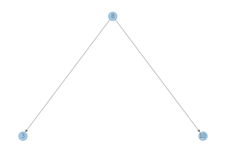
    nx.draw(G, pos, labels=labels, alpha=0.4)

draw_tree(tree)

Search#

Given a tree and a target value, how do we determine whether the target is in the tree?

Start at the root. If you find the target, stop.
If the target is less than the value at the root, go left.
If the target is greater than the value at the root, go right.
If you get to a non-existent node, stop.

Exercise: Write a function called search that takes a BSTree and a target value and returns True if the target value appears in the tree.

Exercise: Many tree operations lend themselves to recursive implementations. Write a function called search_rec that searches the tree recursively.

Hint: Start with a copy of is_bst.

Insert#

The point of the BST is that we can add and remove elements efficiently, compared to a sorted array.

So let’s see what that looks like.

def insert(tree, data):
    tree.root = insert_node(tree.root, data)
    
def insert_node(node, data):
    if node is None:
        return Node(data)
    
    if data < node.data:
        node.left = insert_node(node.left, data)
    else:
        node.right = insert_node(node.right, data)
        
    return node

We’ll test it by starting with an empty tree and adding elements one at a time.

tree = BSTree()

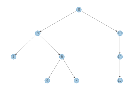
values = [8, 3, 10, 1, 6, 14, 4, 7, 13]
for value in values:
    insert(tree, value)

tree

BSTree(Node(8, Node(3, Node(1, None, None), Node(6, Node(4, None, None), Node(7, None, None))), Node(10, None, Node(14, Node(13, None, None), None))))

draw_tree(tree)

If things have gone according to plan, the result should be a BST.

is_bst(tree)

True

Sorting#

If we traverse the tree recursively and print the elements as we go, we get the values in sorted order.

def print_tree(tree):
    print_tree_rec(tree.root)
    
def print_tree_rec(node):
    if node is None:
        return
    
    print_tree_rec(node.left)
    print(node.data, end=' ')
    print_tree_rec(node.right)

print_tree(tree)

1 3 4 6 7 8 10 13 14

Exercise: Write a generator method called iterate_tree that traverses the tree and yields the elements in order.

You can do this iteratively or recursively.

Badness 10000#

If the tree is reasonably well balanced, the height is proportional to log n, where n is the number of elements.

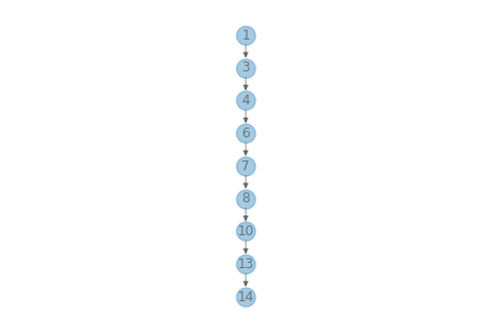
But let’s see what happens if we add elements in sorted order.

tree3 = BSTree()
for x in sorted(values):
    insert(tree3, x)

draw_tree(tree3)

Now traversing the tree takes linear time. To avoid this problem, there are variations of BST that are self-balancing.

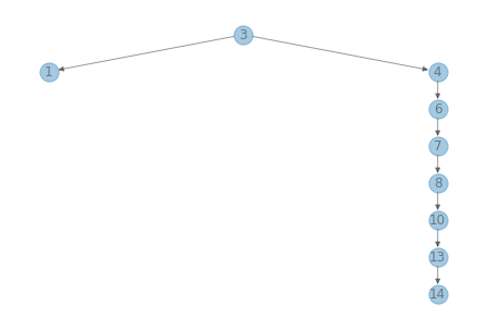
Most are based on tree rotation operations. For example, the following is a function that rotates a tree to the left (following Wikipedia’s nomenclature for what “left” and “right” mean).

def rotate_left(node):
    if node is None or node.right is None:
        return node

    pivot = node.right
    node.right = pivot.left
    pivot.left = node
    
    return pivot

tree3.root = rotate_left(tree3.root)
draw_tree(tree3)

Data Structures and Information Retrieval in Python

License: Creative Commons Attribution-NonCommercial-ShareAlike 4.0 International

Data Structures and Information Retrieval in Python

Search

Contents

Search#

Linear Search#

Bisection#

Binary search tree#

Draw the Tree#

Search#

Insert#

Sorting#

Badness 10000#