The Distribution of U.S. Firm Revenue

In a previous example, I fit several models to the distribution of firm sizes measured by number of employees, using COMPUSTAT data. And in another example, I fit the same models to the distribution of revenue for French companies.

In this example, I’ll use the same COMPUSTAT data, but measure firm size by revenue, and fit the same models in the same way.

Click here to run this notebook on Colab.

Show code cell content

Hide code cell content

import pandas as pd
import numpy as np
import matplotlib.pyplot as plt

from empiricaldist import Cdf, TailDist
from utils import decorate, set_pyplot_params

set_pyplot_params()

Data

Bloom, Nicholas, Jones, Charles I., Van Reenen, John, and Webb, Michael. Data and Code for: Are Ideas Getting Harder to Find?: Compustat: Compustat WRDS 2016 06 13.csv. Nashville, TN: American Economic Association [publisher], 2020. Ann Arbor, MI: Inter-university Consortium for Political and Social Research [distributor], 2020-03-30. https://doi.org/10.3886/E111743V2-209061

The extract is distributed with the openICPSR replication archive under CC BY 4.0, so we can redistribute it here. Individual firms count as research subjects under ICPSR rules, so we report only aggregate distributional results and do not identify particular companies.

COMPUSTAT reports two measures of revenue, sale and revt. Where both are reported, they are the same, but revt is available for more firms, so I’ll use it. Revenue is reported in millions, in the currency the firm reports in, which is either U.S. or Canadian dollars.

Show code cell content

Hide code cell content

year = 2014
df = raw.loc[(raw["fyear"] == year) & (raw["revt"] > 0), ["fyear", "revt", "curcd"]].copy()
df["curcd"].value_counts()

curcd
USD    7584
CAD    1113
Name: count, dtype: int64

To convert Canadian dollars to U.S. dollars, I’ll use the annual average exchange rate from the Federal Reserve (H.10, FRED series AEXCAUS), which is the number of Canadian dollars per U.S. dollar. I use the rate for the calendar year that matches the fiscal year, so for firms whose fiscal year ends early in the calendar year, the conversion is approximate.

The following function converts revenue to U.S. dollars.

Show code cell content

Hide code cell content

def revenue_usd(frame):
    """Revenue in U.S. dollars.

    frame: DataFrame with columns fyear, revt (millions), and curcd

    returns: Series
    """
    rate = frame["fyear"].map(cad_per_usd).where(frame["curcd"] == "CAD", 1.0)
    return frame["revt"] * 1e6 / rate

Show code cell content

Hide code cell content

revenue = revenue_usd(df)
n = len(revenue)
revenue.describe()

count    8.697000e+03
mean     3.849256e+09
std      1.711566e+10
min      9.055510e+02
25%      3.069000e+07
50%      2.302250e+08
75%      1.433400e+09
max      4.835210e+11
dtype: float64

As with employment, the mean is far above what we would expect for all U.S. firms, because COMPUSTAT is dominated by large, mostly publicly traded companies.

Distribution of revenue

Here is the CDF of revenue on a log-\(x\) scale.

Show code cell source

Hide code cell source

Cdf.from_seq(revenue).plot()

decorate(xlabel="Revenue (US dollars)", ylabel="CDF", xscale="log",
         title=f"COMPUSTAT revenue, {year}")

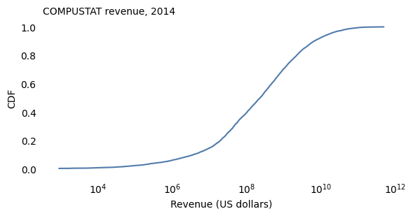
On a log scale, the CDF has roughly the sigmoid shape of a normal distribution, so the lognormal model is a natural candidate.

Log revenue

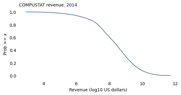
As in the other examples, I’ll work with the logarithm of revenue, base 10.

Show code cell content

Hide code cell content

mags = np.log10(revenue)
mags.describe()

count    8697.000000
mean        8.252025
std         1.314951
min         2.956913
25%         7.486997
50%         8.362152
75%         9.156367
max        11.684415
dtype: float64

Show code cell content

Hide code cell content

tail_log = TailDist.from_seq(mags)

Show code cell content

Hide code cell content

xlabel_log = "Revenue (log10 US dollars)"
ylabel = "Prob >= $x$"

Show code cell source

Hide code cell source

tail_log.plot()

decorate(xlabel=xlabel_log, ylabel=ylabel, title=f"COMPUSTAT revenue, {year}")

Fitting truncated models

As in the employment example, I’ll treat the smallest value in the sample as a cutoff and truncate each model there, and fit the models using functions in tail_models.py:

• Location and scale are chosen to match percentiles of the data (fit_loc_scale).

• A shape parameter, if the model has one, is chosen to match the largest values – it minimizes the squared differences between the logarithms of the tail probabilities, from 1% down to the second-largest value (fit_shape).

plot_two shows the data and a model on a linear-\(y\) scale and a log-\(y\) scale; on the log-\(y\) scale, the shaded area shows how much variation we would expect due to sampling if the model were correct. model_errors computes the mean absolute difference between the tail distributions on the linear scale and the root mean squared difference between log tail probabilities.

Show code cell content

Hide code cell content

from tail_models import (
    truncated_tail,
    fit_loc_scale,
    fit_shape,
    pareto2_tail,
    fit_pareto2_scale,
    fit_pareto2_alpha,
    plot_two,
    model_errors,
    fit_models,
    YTICKS_LOG,
)

Show code cell content

Hide code cell content

low, high = tail_log.qs.min(), tail_log.qs.max()
qs = np.linspace(low, high + 0.5, 2000)
log_cutoff = low

Show code cell content

Hide code cell content

results = {}

Lognormal model

Show code cell content

Hide code cell content

from scipy.stats import norm

mu, sigma = fit_loc_scale(norm, tail_log, ps=np.linspace(0.1, 0.99, 20))
mu, sigma

(8.327402224696566, 1.2465792684700328)

Show code cell source

Hide code cell source

tail_lognormal = truncated_tail(norm, qs, mu, sigma)
plot_two(tail_log, tail_lognormal, n, "lognormal model", xlabel_log)

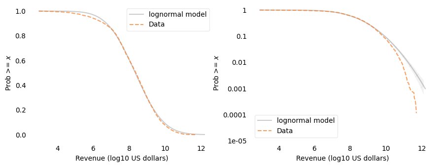
On the linear-\(y\) scale, the lognormal model fits well above about $10 million; below that, the data are below the model, which means there are more firms with very small revenue than the model predicts. On the log-\(y\) scale, above about $10 billion, the data fall below the model, and for the largest firms the discrepancy is up to an order of magnitude – well outside the range we would expect from random sampling. As with employment, the largest firms are less common than the lognormal model predicts.

Show code cell content

Hide code cell content

results["lognormal"] = model_errors(tail_log, tail_lognormal)
results["lognormal"]

(0.008493945798591708, 0.5401525224853155)

Log-Student-\(t\) model

The Student-\(t\) distribution has a parameter, df, that controls the thickness of the tails; a log-Student-\(t\) model can only have thicker tails than the lognormal model.

Show code cell content

Hide code cell content

from scipy.stats import t as t_dist

df_t = fit_shape(t_dist, tail_log, shape0=10, bounds=(1, 1000))
df_t

999.9993027032061

Show code cell content

Hide code cell content

mu_t, sigma_t = fit_loc_scale(t_dist, tail_log, shape=(df_t,))
mu_t, sigma_t

(8.327788809477802, 1.2411318557168631)

Show code cell source

Hide code cell source

tail_t = truncated_tail(t_dist, qs, df_t, mu_t, sigma_t)
plot_two(tail_log, tail_t, n, "log-t model", xlabel_log)

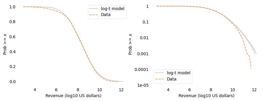
As with employment, the fitted value of df is at the upper bound of the search, 1000, so the best log-\(t\) model is indistinguishable from the lognormal model: these data need thinner tails, not thicker ones.

Show code cell content

Hide code cell content

results["log-t"] = model_errors(tail_log, tail_t)
results["log-t"]

(0.008429556782407274, 0.5352198028520144)

Log-generalized-normal model

The generalized normal distribution has a shape parameter, \(\beta\): \(\beta = 2\) is the normal distribution, \(\beta < 2\) has thicker tails, and \(\beta > 2\) has thinner tails.

Show code cell content

Hide code cell content

from scipy.stats import gennorm

beta = fit_shape(gennorm, tail_log, shape0=2, bounds=(0.5, 20))
beta

2.8911929751088166

Show code cell content

Hide code cell content

mu_g, alpha_g = fit_loc_scale(gennorm, tail_log, shape=(beta,))
mu_g, alpha_g

(8.3254550915095, 1.8643986717383727)

Show code cell source

Hide code cell source

tail_gennorm = truncated_tail(gennorm, qs, beta, mu_g, alpha_g)
plot_two(tail_log, tail_gennorm, n, "log-gennorm model", xlabel_log)

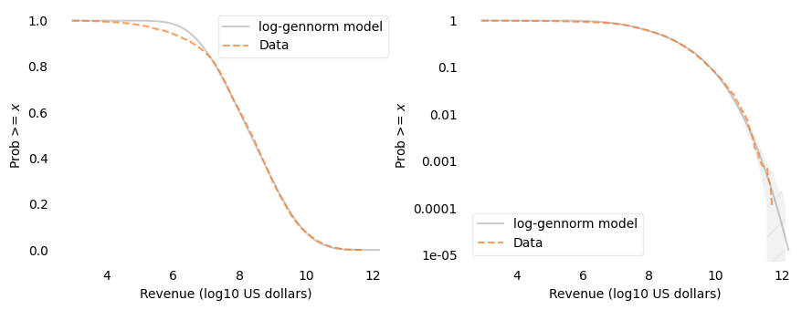
The fitted value of \(\beta\) is about 2.9, greater than 2, so the departure from the lognormal model is toward thinner tails. On the log-\(y\) scale, the log-generalized-normal model fits well, with the data within the range we would expect from random sampling. On the linear-\(y\) scale, it has the same discrepancy below $10 million as the lognormal model.

Show code cell content

Hide code cell content

results["log-gennorm"] = model_errors(tail_log, tail_gennorm)
results["log-gennorm"]

(0.00853412336377755, 0.06402911040379779)

Pareto model

As in the other examples, I’ll use a Pareto II (Lomax) distribution, which has an exponent, \(\alpha\), and a scale parameter, \(s\):

\[P(X \ge x ~|~ X \ge c) = \left(1 + \frac{x - c}{s}\right)^{-\alpha}\]

where \(c\) is the cutoff. fit_pareto2_alpha chooses \(\alpha\) to match the largest values, and fit_pareto2_scale chooses the scale to match percentiles.

Show code cell content

Hide code cell content

alpha = fit_pareto2_alpha(tail_log, log_cutoff)
alpha

0.8854771654818054

Show code cell content

Hide code cell content

log_scale = fit_pareto2_scale(tail_log, alpha, log_cutoff)
log_scale, 10**log_scale

(8.263355922375098, 183381669.56860912)

Show code cell source

Hide code cell source

tail_pareto = pareto2_tail(qs, alpha, log_scale, log_cutoff)
plot_two(tail_log, tail_pareto, n, "Pareto II model", xlabel_log)

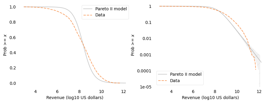
The fitted exponent is about 0.89, and the scale is about $180 million. The Pareto II model does not fit this distribution: on the linear-\(y\) scale it is visibly off over most of the range, and on the log-\(y\) scale it is below the data between about $100 million and $100 billion and above the data for the largest firms.

Show code cell content

Hide code cell content

results["Pareto II"] = model_errors(tail_log, tail_pareto)
results["Pareto II"]

(0.07630993168613927, 0.31305324509418075)

Comparison

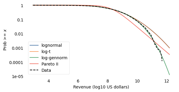
Here are all four models on a log-\(y\) scale.

Show code cell source

Hide code cell source

tail_lognormal.plot(label="lognormal")
tail_t.plot(label="log-t")
tail_gennorm.plot(label="log-gennorm")
tail_pareto.plot(label="Pareto II")
tail_log.plot(color="black", ls="--", label="Data")

decorate(xlabel=xlabel_log, ylabel=ylabel, yscale="log", ylim=[1e-5, 1.5])
plt.yticks(YTICKS_LOG, YTICKS_LOG);

And here are the errors.

Show code cell source

Hide code cell source

pd.DataFrame(results, index=["Mean abs error", "RMS log error"]).T.round(4)

	Mean abs error	RMS log error
lognormal	0.0085	0.5402
log-t	0.0084	0.5352
log-gennorm	0.0085	0.0640
Pareto II	0.0763	0.3131

The lognormal and log-\(t\) curves are nearly the same. On the linear scale, the lognormal, log-\(t\), and log-generalized-normal models have about the same error; the Pareto II model’s error is about nine times larger. On the log scale, the log-generalized-normal model has the smallest error by a wide margin.

Robustness

To see whether these results depend on the year or the cutoff, I’ll fit the lognormal, log-generalized-normal, and Pareto II models for each fiscal year from 2005 through 2014, and for several cutoffs. The following function selects the data, converting Canadian dollars at the rate for each year.

Show code cell content

Hide code cell content

def select_revenue(raw, year, cutoff):
    """Select log revenue (US dollars) at or above the cutoff for one fiscal year."""
    frame = raw.loc[(raw["fyear"] == year) & (raw["revt"] > 0)]
    revenue = revenue_usd(frame)
    return np.log10(revenue[revenue >= cutoff])

Here are the results for each year, using all firms with positive revenue. With no cutoff argument, fit_models uses the smallest value as the cutoff.

Show code cell source

Hide code cell source

rows = {y: fit_models(select_revenue(raw, y, 0)) for y in range(2005, 2015)}
by_year = pd.DataFrame(rows).T
by_year.round(3)

	n	beta	alpha	log_scale	rmse_lognormal	rmse_gennorm	rmse_pareto
2005	10194.0	2.409	0.895	8.076	0.342	0.094	0.314
2006	9924.0	2.409	0.888	8.117	0.349	0.115	0.322
2007	9454.0	2.421	0.877	8.147	0.355	0.135	0.331
2008	9180.0	2.394	0.883	8.179	0.327	0.099	0.308
2009	9040.0	2.413	0.884	8.146	0.354	0.157	0.341
2010	8918.0	2.445	0.877	8.180	0.366	0.131	0.329
2011	8814.0	2.515	0.870	8.207	0.386	0.098	0.313
2012	9107.0	2.665	0.854	8.153	0.466	0.081	0.318
2013	9101.0	2.761	0.857	8.168	0.498	0.072	0.318
2014	8697.0	2.891	0.885	8.263	0.540	0.064	0.313

In every year from 2005 through 2014, the log-generalized-normal model fits best on the log scale, with \(\beta\) between 2.4 and 2.9 – always thinner-tailed than the lognormal model. The fitted value of \(\beta\) increases after 2010. The lognormal and Pareto II models fit substantially worse in every year, and the Pareto exponent is between 0.85 and 0.90.

And here are the results for fiscal year 2014 with several cutoffs.

Show code cell source

Hide code cell source

cutoffs = [1e6, 1e7, 1e8, 1e9]
rows = {f"${c:,.0f}": fit_models(select_revenue(raw, year, c), np.log10(c)) for c in cutoffs}
by_cutoff = pd.DataFrame(rows).T
by_cutoff.round(3)

	n	beta	alpha	log_scale	rmse_lognormal	rmse_gennorm	rmse_pareto
$1,000,000	8190.0	2.645	0.916	8.378	0.458	0.073	0.300
$10,000,000	7433.0	2.663	0.966	8.544	0.480	0.070	0.282
$100,000,000	5266.0	2.646	1.111	8.999	0.301	0.072	0.228
$1,000,000,000	2569.0	19.999	1.366	9.623	0.323	0.171	0.154

With cutoffs of $1 million, $10 million, and $100 million, the results hardly change: \(\beta\) is about 2.65 and the log-generalized-normal model fits well. So the discrepancy among the smallest firms doesn’t affect the fitted shape.

With the $1 billion cutoff, \(\beta\) reaches the upper bound of the search, 20, so that fit is not meaningful. The Pareto II exponent increases with the cutoff, from about 0.92 to about 1.37, and with the $1 billion cutoff the Pareto II model fits a little better than the others – but among these roughly 2,600 firms, none of the models fits as well as the log-generalized-normal model does for the whole sample.

Summary

• For COMPUSTAT revenue in 2014, the lognormal model fits most of the distribution, but the largest firms are less common than it predicts – the same pattern as for employment.

• A log-Student-\(t\) model can’t help, because it can only make the tails thicker.

• A log-generalized-normal model with \(\beta\) about 2.9 fits the upper part of the distribution well, and it fits best on the log scale in every year from 2005 through 2014, with \(\beta\) between 2.4 and 2.9. The fitted shape is about the same for cutoffs from $1 million to $100 million.

• A Pareto II model does not fit the whole sample; above $1 billion it does a little better than the others, with exponent about 1.4.

Copyright 2026 Allen B. Downey

Example related to Chapters 4 and 8 from Probably Overthinking It.

License: Attribution-NonCommercial-ShareAlike 4.0 International (CC BY-NC-SA 4.0)