The Long Tail of Disaster#
Probably Overthinking It is available from Bookshop.org and Amazon (affiliate links).
Click here to run this notebook on Colab.
You would think we’d be better prepared for disaster. But events like Hurricane Katrina in 2005, which caused catastrophic flooding in New Orleans, and Hurricane Maria in 2017, which caused damage in Puerto Rico that has still not been repaired, show that large-scale disaster response is often inadequate. Even wealthy countries – with large government agencies that respond to emergencies and well-funded organizations that provide disaster relief – have been caught unprepared time and again.
There are many reasons for these failures, but one of them is that rare, large events are fundamentally hard to comprehend. Because they are rare, it is hard to get the data we need to estimate precisely how rare. And because they are large, they challenge our ability to imagine quantities that are orders of magnitude bigger than what we experience in ordinary life.
My goal in this chapter is to present the tools we need to comprehend the small probabilities of large events so that, maybe, we will be better prepared next time.
The Distribution of Disaster#
Natural and human-caused disasters are highly variable. The worst disasters, in terms of both lives lost and property destroyed, are thousands of times bigger than smaller, more common disasters.
That fact might not be surprising, but there is a pattern to these costs that is less obvious. One way to see this pattern is to plot the magnitudes of the biggest disasters on a logarithmic scale. To demonstrate, I’ll use the estimated costs from a list of 125 disasters on Wikipedia.
# If you want a more recent list, try this, but it might not work if the
# page has been reorganized.

# download("https://en.wikipedia.org/wiki/List_of_disasters_by_cost")
tables = pd.read_html(filename)
disasters = tables[0]
disasters.head()
| Cost ($billions) | Fatalities | Event | Type | Year | Nation | ||
|---|---|---|---|---|---|---|---|
| Unnamed: 0_level_1 | (2021)[5] | Fatalities | Event | Type | Year | Nation | |
| 0 | $700[2] | $774.9 (2021) | 4000 - 200000[6] | Chernobyl disaster [1] | Contamination (Radioactive) | 1986 | Soviet Union (, ) |
| 1 | $360[7][8][4] | $423.7 (2021) | 19747 | 2011 Tōhoku earthquake and tsunami | Earthquake, Tsunami, Contamination (Radioactive) | 2011 | Japan |
| 2 | $197[9] | $344.7 (2021) | 5502 – 6434 | Great Hanshin earthquake | Earthquake | 1995 | Japan |
| 3 | $148[10] | $179.7 (2021) | 87587 | 2008 Sichuan earthquake | Earthquake | 2008 | China |
| 4 | $125[11] | $167.4 (2021) | 1245 – 1836 | Hurricane Katrina | Tropical cyclone | 2005 | United States |
Most of the disasters on the list are natural, including 56 tropical cyclones and other windstorms, 16 earthquakes, 8 wildfires, 8 floods, and 6 tornadoes. The costliest natural disaster on the list is the 2011 Tōhoku earthquake and tsunami, which caused the Fukushima nuclear disaster, with a total estimated cost of $424 billion in 2021 dollars.
There are not as many human-made disasters on the list, but the costliest is one of them: the Chernobyl disaster, with an estimated cost of $775 billion. The list of human-made disasters includes four other instances of contamination with oil or radioactive material, three space flight accidents, two structural failures, two explosions, and two terror attacks.
This list is biased: disasters that affect wealthy countries are more likely to damage high-value assets, and the reckoning of the costs is likely to be more complete. A disaster that affects more lives – and more severely – in other parts of the world might not appear on the list. Nevertheless, it provides a way to quantify the sizes of some large disasters.
disasters["Type", "Type"].value_counts()
(Type, Type)
Tropical cyclone                                    49
Earthquake                                          16
Wildfire                                             8
Flood                                                8
European windstorm                                   7
Tornado                                              6
Space flight accident                                3
Drought                                              3
Hailstorm                                            3
Structure failure                                    2
Contamination (Oil)                                  2
Terror attack                                        2
Volcano                                              2
Winter storm                                         2
Explosion                                            2
Contamination (Radioactive)                          1
Contamination (Radiation)                            1
Maritime disaster                                    1
Severe Thunderstorm                                  1
Drought, Wildfire                                    1
Severe storm                                         1
Earthquake, Tsunami, Contamination (Radioactive)     1
Earthquake, Tsunami                                  1
Winter storm, power outage                           1
Fire                                                 1
Name: count, dtype: int64
Some of the costs are reported as a range, so I compute the midpoints.
costs = disasters["Cost ($billions)", "(2021)[5]"].str.split()
costs[0] = 774.9
costs[11] = (72.2 + 120.4) / 2
costs[13] = (56.9 + 64.4) / 2
costs[25] = (32.2 + 199.1) / 2
costs[35] = (27.1 + 36.1) / 2
costs[44] = (18.3 + 29.8) / 2
costs[49] = (10.9 + 16.4) / 2
costs[62] = (9.8 + 17.0) / 2
costs[111] = (1.8 + 2.8) / 2
costs[119] = (4.1 + 5.6) / 2
disasters[costs.isna()]
| Cost ($billions) | Fatalities | Event | Type | Year | Nation | ||
|---|---|---|---|---|---|---|---|
| Unnamed: 0_level_1 | (2021)[5] | Fatalities | Event | Type | Year | Nation | |
Remove the dollar signs and convert to float.
xs = []
for cost in costs:
    try:
        x = float(cost[0].strip("$"))
    except:
        x = cost
    assert type(x) is float
    xs.append(x)

xs.sort(reverse=True)
Get the magnitudes and ranks
mags = np.log10(xs)
n = len(mags)
ranks = np.arange(1, n + 1)
The following figure shows a “rank-size plot” of the data: the x-axis shows the ranks of the disasters from 1 to 125, where 1 is the most costly; the y-axis shows their costs in billions of U.S. dollars.
plt.plot(ranks, xs)
decorate(
    xlabel="Rank (1 to 125)",
    ylabel="Cost (billions of 2021 dollars)",
    xscale="log",
    yscale="log",
    title="Rank-size plot for cost of disasters",
)
xticks = [1, 2, 5, 10, 20, 50, 100]
yticks = [1, 10, 100, 1000]
plt.xticks(xticks, xticks)
plt.yticks(yticks, yticks)
savefig("longtail1.png")
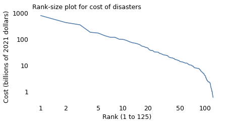
With both axes on a log scale, the rank-size plot is a nearly straight line, at least for the top 100 disasters. And the slope of this line is close to 1, which implies that each time we double the rank, we cut the costs by one half. That is, compared to the costliest disaster, the cost of the second-worst is one half; the cost of the fourth-worst is one quarter; the cost of the eighth is one eighth, and so on.
index = np.array([1, 2, 4, 8, 16, 32, 64]) - 1
steps = 10 ** mags[index]
steps /= steps[0]
1 / steps
array([ 1.        ,  1.82888836,  4.31218698,  6.70038911, 12.77658697,
       31.62857143, 74.50961538])
In this chapter I will explain where this pattern comes from, but I’ll warn you that the answers we have are incomplete. There are several ways that natural and engineered systems can generate distributions like this. In some cases, like impact craters and the asteroids that form them, we have physical models that explain the distribution of their sizes. In other cases, like solar flares and earthquakes, we only have hints.
We will also use this pattern to make predictions. To do that, we have to understand “long-tailed” distributions. In Chapter 1 we saw that many measurements, like human height, follow a Gaussian distribution. And in Chapter 4 we saw that many other measurements, like human weight, follow a lognormal distribution. I suggested a general explanation for these patterns:
If the things we measure are the result of adding many factors, the sum tends to be Gaussian.
If the things we measure are the result of multiplying many factors, the product tends to be lognormal.
The difference between these distributions is most noticeable in the tails, that is, in the distribution of the most extreme values. Gaussian distributions are symmetric, and their tails don’t extend far from the mean. Lognormal distributions are asymmetric; usually the tail extends farther to the right than the left, and it extends farther from the mean.
If you think measurements follow a Gaussian distribution, and they actually follow a lognormal distribution, you will be surprised to find outliers much farther from the mean than you expect. That’s why the fastest runners are much faster than ordinary runners and the best chess players are so much better than casual players.
For this reason, the lognormal distribution is considered a “long-tailed” distribution. But it is not the only long-tailed distribution, and some of the others have tails even longer than lognormal.
So, if you think measurements follow a lognormal distribution, and they actually follow one of these “longer than lognormal” distributions, you will be surprised to find outliers much, much farther from the mean than you expect.
Let’s get back to the distribution of disaster sizes, and we’ll see the difference one of these long-tailed distributions can make.
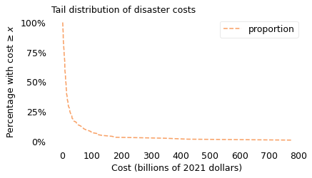
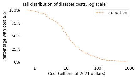
To visualize disaster sizes, I will show the “tail distribution”, which is the complement of the cumulative distribution function (CDF). In Chapter 5, we used a tail distribution to represent survival times for cancer patients. In that context, it shows the fraction of patients that survive a given time after diagnosis. In the context of disasters, it shows the fraction of disasters whose costs exceed a given threshold. The following figure shows the tail distribution of the 125 costliest disasters, on a log scale, along with a lognormal model.
from utils import make_surv, fit_truncated_normal

surv = make_surv(mags)
mu, sigma = fit_truncated_normal(surv)
[1.07816053 0.57668442]
[1.07816055 0.57668442]
[1.07816053 0.57668444]
[1.04133203 0.54825645]
[1.04133204 0.54825645]
[1.04133203 0.54825647]
[1.04293263 0.54534355]
[1.04293265 0.54534355]
[1.04293263 0.54534356]
[1.04292536 0.54517372]
[1.04292537 0.54517372]
[1.04292536 0.54517373]
df = pd.DataFrame(dict(surv=surv))
df.index.name = 'magnitude'
df.reset_index()
| magnitude | surv | |
|---|---|---|
| 0 | -0.221849 | 1.000 |
| 1 | -0.154902 | 0.992 |
| 2 | -0.096910 | 0.984 |
| 3 | 0.000000 | 0.976 |
| 4 | 0.079181 | 0.960 |
| ... | ... | ... |
| 103 | 2.223755 | 0.040 |
| 104 | 2.254548 | 0.032 |
| 105 | 2.537441 | 0.024 |
| 106 | 2.627058 | 0.016 |
| 107 | 2.889246 | 0.008 |
108 rows × 2 columns
df.reset_index().to_csv('disaster_magnitude.csv', index=False)
!head disaster_magnitude.csv
magnitude,surv
-0.22184874961635637,1.0
-0.1549019599857432,0.9920000000000007
-0.09691001300805639,0.9840000000000007
0.0,0.9760000000000006
0.07918124604762482,0.9600000000000006
0.11394335230683678,0.9520000000000006
0.146128035678238,0.9440000000000006
0.20411998265592482,0.9360000000000006
0.2787536009528289,0.9280000000000006
from utils import truncated_normal_sf

low, high = mags.min(), mags.max() * 0.99
qs = np.linspace(low, high, 2000)
surv_model = truncated_normal_sf(qs, mu, sigma)
ylabel = "Percentage with cost ≥ $x$"
xlabel = "Cost (billions of 2021 dollars)"

xlabels = [1, 10, 100, 1000]
xticks = np.log10(xlabels)

yticks = [1, 0.1, 0.01]
ylabels = ["100%", "10%", "1%"]
yticks = np.linspace(1, 0, 5)
ylabels = ["100%", "75%", "50%", "25%", "0%"]
yticks
array([1. , 0.75, 0.5 , 0.25, 0. ])
surv_linear = make_surv(xs)
surv_linear.plot(color="C1", ls="--")

plt.yticks(yticks, ylabels)
decorate(
    xlabel=xlabel, ylabel=ylabel, title="Tail distribution of disaster costs"
)
savefig("longtail1a.png")
surv.plot(color="C1", ls="--")

plt.xticks(xticks, xlabels)
plt.yticks(yticks, ylabels)
decorate(
    xlabel=xlabel, ylabel=ylabel, title="Tail distribution of disaster costs, log scale"
)
savefig("longtail1b.png")
surv_model.plot(color="gray", alpha=0.4, label="Lognormal model")
plot_error_bounds(surv_model, n, color="gray")
surv.plot(color="C1", ls="--", label="Data")

plt.xticks(xticks, xlabels)
plt.yticks(yticks, ylabels)
decorate(
    xlabel=xlabel, ylabel=ylabel, title="Tail distribution of disaster costs, log scale"
)
savefig("longtail2.png")
surv([0, 1, 2])
array([0.976, 0.544, 0.072])
The dashed line shows the fraction of disasters that exceed each magnitude of cost. For example, 98% of the disasters exceed a cost of \(1 billion, 54% exceed \)10 billion, and 7% exceed $100 billion.
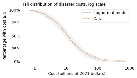
The gray line shows a lognormal model I chose to fit the data; the shaded area shows how much variation we expect with a sample size of 125. Most of the data fall within the bounds of the shaded area, which means that they are consistent with the lognormal model.
However, if you look closely, there are more large-cost disasters than we expect in a lognormal distribution. To see this part of the distribution more clearly, we can plot the y-axis on a log scale; the following figure shows what that looks like.
x = np.log10(500)
y1 = surv(x)
y2 = surv_model(x)
y1 * 1e3, y2 * 1e3, y1 / y2
(15.999999999999897, 1.2081898734673209, 13.24295158515303)
# The Surv object doesn't interpolate, so y1 ends up too high in this example

from scipy.interpolate import interp1d

interp = interp1d(surv.index, surv.values, fill_value="extrapolate")
y1 = interp(x)
plt.plot([x, x], [y1, y2], ls=":", color="gray")

surv_model.plot(color="gray", alpha=0.4, label="Lognormal model")
plot_error_bounds(surv_model, n, color="gray")
surv.plot(color="C2", ls="--", label="Data")
plot_error_bounds(surv_model, n, color="gray")
plt.xticks(xticks, xlabels)
decorate(
    xlabel=xlabel,
    ylabel=ylabel,
    title="Tail distribution of disaster costs, log-log scale",
    yscale="log",
)

yticks = [1, 0.1, 0.01, 0.001]
ylabels = ["100%", "10%", "1%", "0.1%"]
plt.yticks(yticks, ylabels)
savefig("longtail3.png")
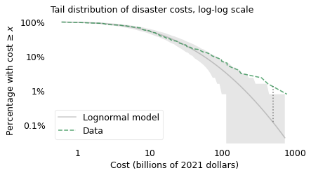
Again, the shaded area shows how much variation we expect in a sample of this size from a lognormal model. In the extreme tail of the distribution, this area is wide because there are only a few observations in this range: where we have less data, we have more uncertainty.
This view of the distribution is like a microscope that magnifies the tail. Now we can see more clearly where the model diverges from the data and by how much. For example, the vertical dotted line shows the discrepancy at $500 billion. According to the model, only 1 out of 1000 disasters should exceed this cost, but the actual rate is 16 per 1000. If your job is to prepare for disasters, an error that large could be, well, disastrous.
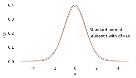
To make better predictions, we need a model that accurately estimates the probability of large disasters. In the literature of long-tailed distributions, there are several to choose from; the one I found that best matches the data is Student’s \(t\)-distribution. It was described in 1908 by William Sealy Gosset, using the pseudonym “Student”, while he was working on statistical problems related to quality control at the Guinness Brewery.
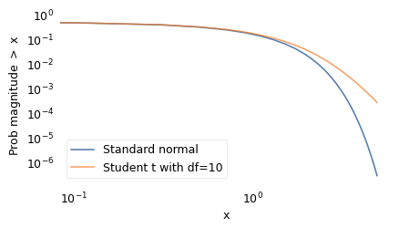
The shape of the \(t\)-distribution is a bell curve similar to a Gaussian, but the tails extend farther to the right and left. It has two parameters that determine the center point and width of the curve, like the Gaussian distribution, plus a third parameter that controls the thickness of the tails, that is, what fraction of the values extend far from the mean.
from scipy.stats import norm
from scipy.stats import t as t_dist

xs = np.linspace(-5, 5, 201)
ys1 = norm.pdf(xs, 0, 1)

plt.plot(xs, ys1, label='Standard normal')

df = 10
ys2 = t_dist.pdf(xs, df, 0, 1)
plt.plot(xs, ys2, label='Student t with df=10')

plt.xlabel('x')
plt.ylabel('PDF')
plt.legend()
plt.tight_layout()
savefig("longtail3a.png")
xs = np.linspace(-5, 5)
ys1 = norm.sf(xs, 0, 1)

plt.plot(xs, ys1, label='Standard normal')

ys2 = t_dist.sf(xs, df, 0, 1)
plt.plot(xs, ys2, label='Student t with df=10')

plt.xlabel('x')
plt.ylabel('Prob magnitude $>$ x')
plt.xscale('log')
plt.yscale('log')
plt.legend()
plt.tight_layout()
savefig("longtail3b.png")
Since I am using a \(t\)-distribution to fit the logarithms of the values, I’ll call the result a log-\(t\) model. The following figures shows the distribution of costs again, along with a log-\(t\) model I chose to fit the data. In the top figure, the y-axis shows the fraction of disasters on a linear scale; in the bottom figure, the y-axis shows the same fractions on a log scale.
from utils import minimize_df

df = minimize_df(5, surv, [(0, 20)])
from utils import fit_truncated_t

mu, sigma = fit_truncated_t(df, surv)
df, mu, sigma
(array([3.52824501]), 1.0165307353889603, 0.488752041667769)
from utils import truncated_t_sf

low, high = surv.qs.min(), surv.qs.max()
qs = np.linspace(low, high, 2000)
surv_model2 = truncated_t_sf(qs, df, mu, sigma)
model_label = "Log-$t$ model"
ylabel = "Fraction with cost ≥ x"
yticks = [1, 0.1, 0.01]
ylabels = yticks
axs = plot_two(
    surv,
    surv_model2,
    n,
    hatch="/",
    title="Tail distribution of disaster costs with log-$t$ model",
)
savefig("longtail4.png")
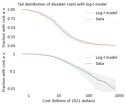
In the top figure, we see that the data fall within the shaded area over the entire range of the distribution. In the bottom figure, we see that the model fits the data well even in the extreme tail.
The agreement between the model and the data provides a hint about why the distribution might have this shape. Mathematically, Student’s \(t\) distribution is a mixture of Gaussian distributions with different standard deviations.
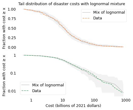
The following figure was not included in the book, but it shows that if we generate values from Gaussian distributions with different standard deviations (drawn from an inverse gamma distribution), the values follow a t distribution.
from scipy.stats import invgamma

np.random.seed(17)

a = df
sigma = np.sqrt(invgamma(a).rvs(size=125))
sigma.mean(), sigma.std()
(0.6007941329583358, 0.1717044227431617)
from scipy.stats import norm

mu = 1.04
sample = norm(mu, sigma).rvs()
surv_sample = make_surv(sample[sample > -0.4])
model_label = "Mix of lognormal"
axs = plot_two(
    surv,
    surv_sample,
    n,
    title="Tail distribution of disaster costs with lognormal mixture",
)
decorate(ylim=[5e-3, 1.1])
savefig("longtail5.png")
Earthquakes#
To describe the magnitudes of earthquakes, I downloaded data from the Southern California Earthquake Data Center. Their archive goes all the way back to 1932, but the sensors they use and their coverage have changed over that time. For consistency, I selected data from January 1981 to April 2022, which includes records of 791,329 earthquakes.
For information on catalog completeness and data sources, see http://www.data.scec.org/about/data_avail.html.
quake_df = pd.read_csv(filename, low_memory=False)
quake_df.shape
(803451, 4)
The magnitude of an earthquake is measured on the “moment magnitude scale”, which is an updated version of the more well-known Richter scale. A moment magnitude is proportional to the logarithm of the energy released by an earthquake. A two-unit difference on this scale corresponds to a factor of 1000, so a magnitude 5 earthquake releases 1000 times more energy than a magnitude 3 earthquake and 1000 times less energy than a magnitude 7 earthquake.
quake_df.head()
| #YYY | MM | DD | MAG | |
|---|---|---|---|---|
| 0 | 1981 | 1 | 1 | 2.3 |
| 1 | 1981 | 1 | 1 | 2.3 |
| 2 | 1981 | 1 | 1 | 2.4 |
| 3 | 1981 | 1 | 1 | 1.6 |
| 4 | 1981 | 1 | 1 | 1.9 |
quake_df.tail()
| #YYY | MM | DD | MAG | |
|---|---|---|---|---|
| 803446 | 2022 | 12 | 31 | 0.5 |
| 803447 | 2022 | 12 | 31 | 1.0 |
| 803448 | 2022 | 12 | 31 | 0.9 |
| 803449 | 2022 | 12 | 31 | 0.6 |
| 803450 | 2022 | 12 | 31 | 0.6 |
year = quake_df["#YYY"] == "1989"
year.sum()
0
quake_df.sort_values(by="MAG").tail(10)
| #YYY | MM | DD | MAG | |
|---|---|---|---|---|
| 102346 | 1987 | 11 | 24 | 6.2 |
| 163645 | 1992 | 6 | 28 | 6.3 |
| 674787 | 2019 | 7 | 4 | 6.4 |
| 408783 | 2003 | 12 | 22 | 6.5 |
| 102647 | 1987 | 11 | 24 | 6.6 |
| 224869 | 1994 | 1 | 17 | 6.7 |
| 335296 | 1999 | 10 | 16 | 7.1 |
| 678320 | 2019 | 7 | 6 | 7.1 |
| 492576 | 2010 | 4 | 4 | 7.2 |
| 163589 | 1992 | 6 | 28 | 7.3 |
mags = quake_df["MAG"]
mags.describe()
count    803451.000000
mean          1.388616
std           0.658252
min           0.000000
25%           0.900000
50%           1.300000
75%           1.800000
max           7.300000
Name: MAG, dtype: float64
(mags < 2).mean()
0.8159564180018446
quake_df.groupby("#YYY")["MAG"].count().iloc[1:-1].describe()
count       40.000000
mean     19397.050000
std      11049.695313
min      10092.000000
25%      13467.500000
50%      16186.000000
75%      20463.000000
max      63571.000000
Name: MAG, dtype: float64
n = mags.count()
n
803451
surv = make_surv(mags)
mu, sigma = fit_truncated_normal(surv)
[1.48860875 0.65822228]
[1.48860877 0.65822228]
[1.48860875 0.6582223 ]
[1.37983937 0.66707222]
[1.37983939 0.66707222]
[1.37983937 0.66707224]
[1.38099766 0.65403304]
[1.38099768 0.65403304]
[1.38099766 0.65403305]
[1.38080268 0.65402889]
[1.3808027  0.65402889]
[1.38080268 0.65402891]
low, high = mags.min(), mags.max() * 0.99
qs = np.linspace(low, high, 2000)
surv_model = truncated_normal_sf(qs, mu, sigma)
The following figure shows the distribution of moment magnitudes compared to a Gaussian model, which is a lognormal model in terms of energy.
x = 4
y1 = surv(x)
y2 = surv_model(x)
xlabel = "Magnitude (log energy)"
ylabel = "Fraction with mag ≥ $x$"
xticks = np.arange(8)
xlabels = xticks
yticks = [1, 0.1, 0.01, 1e-3, 1e-4, 1e-5, 1e-6, 1e-7]
ylabels = [1, 0.1, 0.01, 0.001, "$10^{-4}$", "$10^{-5}$", "$10^{-6}$", "$10^{-7}$"]
model_label = "Lognormal model"
cutoff = surv_model > 2e-7
axs = plot_two(
    surv,
    surv_model[cutoff],
    n,
    title="Earthquake magnitudes with lognormal model",
)
plt.plot([x, x], [y1, y2], ls=":", color="gray")

plt.tight_layout()
savefig("longtail6.png")
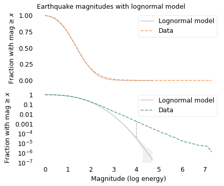
If you only look at the top figure, you might think the lognormal model is good enough. But the probabilities for magnitudes greater than 3 are so small that differences between the model and the data are not visible.
The bottom figure, with the y-axis on a log scale, shows the tail more clearly. Here we can see that the lognormal model drops off more quickly than the data. According to the model, the fraction of earthquakes with magnitude 4 or more should be about 33 per million. But the actual fraction of earthquakes this big is about 1800 per million, more than 50 times higher.
For larger earthquakes, the discrepancy is even bigger. According to the model, fewer than one earthquake in a million should exceed magnitude 5; in reality, about 170 per million do. If your job is to predict large earthquakes, and you underestimate their frequency by a factor of 170, you are in trouble.
The following figures show the same distribution compared to a log-\(t\) model.
y1 * 1e6, y2 * 1e6, y1 / y2
(1784.8008154824963, 31.897268299459753, 55.9546604030893)
x = 5
surv(x) * 1e6, surv_model(x) * 1e7
(168.02518137406247, 0.15958924021795134)
x = 7
surv(x) * 1e6, surv_model(x) * 1e18

# 6.318484473557436, 4.618502751454663
(6.223154865724416, 4.406280129716829)
df = minimize_df(10, surv, [(0, 20)])
mu, sigma = fit_truncated_t(df, surv)
df, mu, sigma
(array([9.07638598]), 1.3634555603669711, 0.6375531964799466)
from scipy.stats import t as t_dist

y7, y8, y9 = t_dist(df, mu, sigma).sf([7, 8, 9])
quakes_per_year = quake_df.groupby("#YYY")["MAG"].count().mean()
quakes_per_year
19129.785714285714
y522 = 1 / 522 / quakes_per_year
y522
1.0014272197675095e-07
low, high = surv.qs.min(), surv.qs.max()
qs = np.linspace(low, 1.1 * high, 2000)
surv_model2 = truncated_t_sf(qs, df, mu, sigma)
model_label = "Log-$t$ model"
xticks = np.arange(9)
xlabels = xticks
axs = plot_two(
    surv,
    surv_model2,
    n,
    hatch="/",
    title="Earthquake magnitudes with log-$t$ model",
)
#plt.plot(8, y8, "s", color="C0", alpha=0.6)
#plt.plot(8, y522, "o", color="C1", alpha=0.6)

plt.tight_layout()
savefig("longtail7.png")
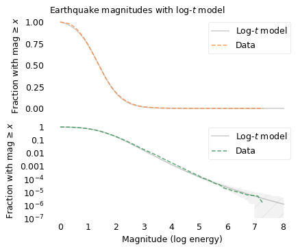
The top figure shows that the log-\(t\) model fits the distribution well for magnitudes less than 3. The bottom figure shows that it also fits the tail of the distribution.
If we extrapolate beyond the data, we can use this model to compute the probability of earthquakes larger than the ones we have seen so far. For example, the square marker shows the predicted probability of an earthquake with magnitude 8, which is about 1.2 per million.
y8 * 1e6
1.197711963360669
1 / quakes_per_year / y8
43.645302435809846
The number of earthquakes in this dataset is about 18,800 per year; at that rate we should expect an earthquake that exceeds magnitude 8 every 43 years, on average. To see how credible that expectation is, let’s compare it to predictions from sources more knowledgeable than me.
In 2015, the U.S. Geological Survey (USGS) published the third revision of the Uniform California Earthquake Rupture Forecast (UCERF3). It predicts that we should expect earthquakes in Southern California that exceed magnitude 8 at a rate of one per 522 years. The circle marker in the figure shows the corresponding probability.
Their forecast is compatible with mine in the sense that it falls within the shaded area that represents the uncertainty of the model. In other words, my model concedes that the predicted probability of a magnitude 8 earthquake could be off by a factor of 10, based on the data we have. Nevertheless, if you own a building in California, or provide insurance for one, a factor of 10 is a big difference. So you might wonder which model to believe, theirs or mine.
To find out, let’s see how their predictions from 2015 have turned out so far. For comparison, I ran the log-\(t\) model again using only data from prior to 2015. The following figure shows their predictions, mine, and the actual number of earthquakes that exceeded each magnitude in the 7.3 years between January 2015 and May 2022.
# https://pubs.usgs.gov/fs/2015/3009/pdf/fs2015-3009.pdf
prefix = quake_df["#YYY"].astype(int) < 2015
quakes_per_year = quake_df.loc[prefix].groupby("#YYY")["MAG"].count().mean()
quakes_per_year
17524.264705882353
mags = quake_df.loc[prefix, "MAG"]
surv = make_surv(mags)
df = minimize_df(10, surv, [(0, 20)])
mu, sigma = fit_truncated_t(df, surv)
df, mu, sigma
(array([8.41547484]), 1.4816444224709593, 0.6026839581707539)
# convert UCERF predictions to quakes per 7.33 years

pred_years = 7.33
ucerf = pred_years / pd.Series([0.24, 2.3, 12, 25, 87, 522], [5, 6, 6.7, 7, 7.5, 8])
ucerf
5.0    30.541667
6.0     3.186957
6.7     0.610833
7.0     0.293200
7.5     0.084253
8.0     0.014042
dtype: float64
# convert log-t predictions to quakes per 7.33 years

a = t_dist(df, mu, sigma).sf(ucerf.index) * quakes_per_year * pred_years
logt = pd.Series(a, ucerf.index)
logt
5.0    20.567019
6.0     3.414845
6.7     1.152932
7.0     0.750355
7.5     0.382366
8.0     0.204125
dtype: float64
# get the actual number of quakes since 2015

suffix = quake_df["#YYY"].astype(int) >= 2015
suffix.sum(), quakes_per_year * pred_years
(207626, 128452.86029411765)
mags = quake_df.loc[suffix, "MAG"]
actual = pd.Series(index=[5, 5.3, 5.7, 6, 6.3, 6.7, 7], dtype=float)
for thresh in actual.index:
    actual[thresh] = (mags > thresh).sum()
actual
5.0    10.0
5.3     7.0
5.7     3.0
6.0     2.0
6.3     2.0
6.7     1.0
7.0     1.0
dtype: float64
x = actual.loc[:7].index
y = actual.loc[:7].values
plt.bar(x, y, width=0.2, color="gray", alpha=0.3, label="actual")
logt.loc[:7].plot(style="s:", alpha=0.6, label="log-$t$")
ucerf.loc[:7].plot(style="o--", alpha=0.6, label="UCERF3")

decorate(xlabel=xlabel, ylabel="Number of quakes", yscale="log")
plt.xticks(x)
yticks = [20, 10, 5, 2, 1, 0.5]
ylabels = yticks
plt.yticks(yticks, yticks)

plt.tight_layout()
savefig("longtail8.png")
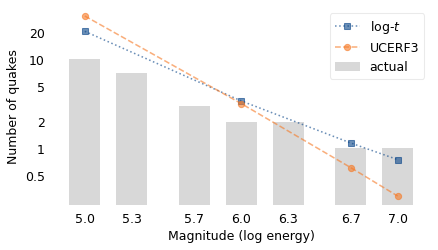
Starting on the left, the UCERF model predicted that there would be 30 earthquakes in this interval with magnitude 5.0 or more. The log-\(t\) model predicted 20. In fact, there were 10. So there were fewer large earthquakes than either model predicted.
Near the middle of the figure, both models predicted 3 earthquakes with magnitude 6.0 or more. In fact, there were two, so both models were close.
On the right, the UCERF model expects 0.3 earthquakes with magnitude 7.0 or more in 7.3 years. The log-\(t\) expects 0.8 earthquakes of this size in the same interval. In fact, there was one: the main shock of the 2019 Ridgecrest earthquake sequence measured 7.1.
# https://en.wikipedia.org/wiki/2019_Ridgecrest_earthquakes
1 / (ucerf / 7.33)
5.0      0.24
6.0      2.30
6.7     12.00
7.0     25.00
7.5     87.00
8.0    522.00
dtype: float64
1 / (logt / 7.33)
5.0     0.356396
6.0     2.146510
6.7     6.357705
7.0     9.768712
7.5    19.170102
8.0    35.909361
dtype: float64
The discrepancy between the two models increases for larger earthquakes. The UCERF model estimates 87 years between earthquakes that exceed 7.5; the log-\(t\) model estimates only 19. The UCERF model estimates 522 years between earthquakes that exceed 8.0; the log-\(t\) model estimates only 36. Again, you might wonder which model to believe.
According to their report, UCERF3 was “developed and reviewed by dozens of leading scientific experts from the fields of seismology, geology, geodesy, paleoseismology, earthquake physics, and earthquake engineering. As such, it represents the best available science with respect to authoritative estimates of the magnitude, location, and likelihood of potentially damaging earthquakes throughout the state.”
On the other hand, my model was developed by a lone data scientist with no expertise in any of those fields. And it is a purely statistical model; it is based on the assumption that the processes that generate earthquakes are obliged to follow simple mathematical models, even beyond the range of the data we have observed.
I’ll let you decide.
Solar Flares#
While we wait for the next big earthquake, let’s consider another source of potential disasters: solar flares.
A solar flare is an eruption of light and other electromagnetic radiation from the atmosphere of the Sun that can last from several seconds to several hours. When this radiation reaches Earth, most of it is absorbed by our atmosphere, so it usually has little effect at the surface. Large solar flares can interfere with radio communication and GPS, and they are dangerous to astronauts, but other than that they are not a serious cause for concern.
However, the same disruptions that cause solar flares also cause coronal mass ejections (CME) which are large masses of plasma that leave the Sun and move into interplanetary space. They are more narrowly directed than solar flares, so not all of them collide with a planet, but if they do, the effects can be dramatic.
As a CME approaches Earth, most of its particles are steered away from the surface by our magnetic field. The ones that enter our atmosphere near the poles are sometimes visible as auroras.
However, very large CMEs cause large-scale, rapid changes in the Earth’s magnetic field. Before the Industrial Revolution, these changes might have gone unnoticed, but in the last few hundred years, we have criss-crossed the surface of the Earth with millions of kilometers of wires. Changes in the Earth’s magnetic field with the magnitude created by a CME can drive large currents through these wires. In 1859, a CME induced enough current in telegraph lines to start fires and shock some telegraph operators. In 1989, a CME caused a large-scale blackout in the electrical grid in Quebec, Canada.
If we are unlucky, a very large CME could cause widespread damage in electrical grids that could take years and trillions of dollars to repair. Fortunately, these risks are manageable. With satellites positioned between the Earth and Sun, we have the ability to detect an incoming CME hours before it reaches Earth. And by shutting down electrical grids for a short time, we should be able to avoid most of the potential damage.
So, on behalf of civilization, we have a strong interest in understanding solar flares and coronal mass ejections.
The Space Weather Prediction Center (SWPC) monitors and predicts solar activity and its effects on Earth. Since 1974 it has operated the Geostationary Operational Environmental Satellite system (GOES). Several of the satellites in this system carry sensors that measure solar flares. Data from these sensors, going back to 1975, is available for download.
Since 1997, these datasets include “integrated flux” – the kind of term science fiction writers love – which measures the total energy from a solar flare that would pass through a given area. The magnitude of this flux is one way to quantify its potential for impact on Earth. This dataset includes measurements from more than 36,000 solar flares. The following figure shows the distribution of their magnitudes compared to a lognormal model.
# Kurtzgesagt https://www.youtube.com/watch?v=oHHSSJDJ4oo
flares_df = pd.read_csv(filename, header=None)
flares = flares_df[0]
flares.shape
(36560,)
mags = np.log10(flares)
mags.describe()
count    36560.000000
mean        -3.058657
std          0.691503
min         -5.022276
25%         -3.537602
50%         -3.080922
75%         -2.619789
max          0.414973
Name: 0, dtype: float64
n = mags.count()
n
36560
surv = make_surv(mags)
mu, sigma = fit_truncated_normal(surv)
[-3.04218419  0.69158557]
[-3.04218423  0.69158557]
[-3.04218419  0.69158559]
[-3.0738114   0.68338351]
[-3.07381145  0.68338351]
[-3.0738114   0.68338353]
[-3.07353797  0.68244264]
[-3.07353802  0.68244264]
[-3.07353797  0.68244265]
low, high = mags.min(), mags.max() * 0.99
qs = np.linspace(low, high, 2000)
surv_model = truncated_normal_sf(qs, mu, sigma)
xlabel = "Integrated flux (Joules / square meter)"
ylabel = "Fraction with flux ≥ $x$"
xticks = np.arange(-5, 1)
xlabels = ["$10^{-5}$", "$10^{-4}$", 0.001, 0.01, 0.1, 1]
yticks = [1, 0.1, 0.01, 1e-3, 1e-4, 1e-5, 1e-6]
ylabels = [1, 0.1, 0.01, 0.001, "$10^{-4}$", "$10^{-5}$", "$10^{-6}$"]
flares.max(), flares.min(), flares.max() / flares.min()
(2.6, 9.5e-06, 273684.2105263158)
cutoff = surv_model > 1e-6
x = 0
y1 = surv(x)
y2 = surv_model(x)
y1 * 1e6, y2 * 1e6, y1 / y2
(218.81838074390188, 3.3991818848706328, 64.37383704527177)
model_label = "Lognormal Model"
axs = plot_two(
    surv, surv_model[cutoff], n,
    title="Tail distribution of solar flare flux with lognormal model"
)
lines = plt.plot([x, x], [y1, y2], ls=":", color="gray")

plt.tight_layout()
savefig("longtail9.png")
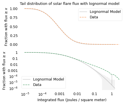
The x-axis shows integrated flux on a log scale; the largest flare observed during this period measured 2.6 Joules per square meter on September 7, 2005. By itself, that number might not mean much, but it is almost a million times bigger than the smallest flare. So the thing to appreciate here is the great range of magnitudes.
Looking at the top figure, it seems like the lognormal model fits the data well. But for fluxes greater than 0.1 Joules per square meter, the probabilities are so small they are indistinguishable.
Looking at the bottom figure, we can see that for fluxes in this range, the lognormal model underestimates the probabilities. For example, according to the model, the fraction of flares with flux greater than 1 should be about 3 per million; in the dataset, it is about 200 per million. The dotted line in the figure shows this difference.
If we are only interested in flares with flux less than 0.01, the lognormal model might be good enough. But for predicting the effect of space weather on Earth, it is the largest flares we care about, and for those the lognormal model might be dangerously inaccurate.
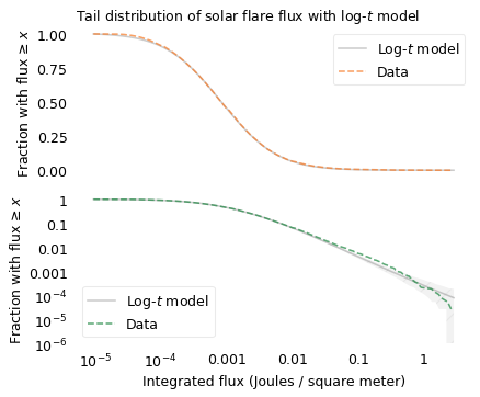
Let’s see if the log-\(t\) model does any better. The following figures show the distribution of fluxes again, along with a log-\(t\) distribution.
df = minimize_df(10, surv, [(0, 20)])
mu, sigma = fit_truncated_t(df, surv)
df, mu, sigma
(array([12.38820488]), -3.0803784847994766, 0.6632850329593064)
low, high = surv.qs.min(), surv.qs.max()
qs = np.linspace(low, 3 * high, 2000)
surv_model2 = truncated_t_sf(qs, df, mu, sigma)
cutoff2 = surv_model2.qs <= 1.1 * high
model_label = "Log-$t$ model"
axs = plot_two(
    surv,
    surv_model2[cutoff2],
    n,
    hatch="/",
    title="Tail distribution of solar flare flux with log-$t$ model",
)

plt.tight_layout()
savefig("longtail10.png")
scale = 10
low, high = surv.qs.min(), surv.qs.max()
qs = np.linspace(low, scale * high, 2000)
surv_model2 = truncated_t_sf(qs, df, mu, sigma)
cutoff2 = surv_model2.qs <= scale * high

xticks = np.arange(-5, 5)
xlabels = ["$10^{-5}$", "$10^{-4}$", 0.001, 0.01, 0.1, 1, 10, 100, 1000, "$10^{5}$"]
yticks = [1, 0.1, 0.01, 1e-3, 1e-4, 1e-5, 1e-6, 1e-7]
ylabels = [1, 0.1, 0.01, 0.001, "$10^{-4}$", "$10^{-5}$", "$10^{-6}$", "$10^{-7}$"]
model_label = "Log-$t$ model"
axs = plot_two(
    surv,
    surv_model2[cutoff2],
    n,
    hatch="/",
    title="Tail distribution of solar flare flux with log-$t$ model",
)

plt.tight_layout()
savefig("longtail10a.png")
The top figure shows that the log-\(t\) model fits the data well over the range of the distribution, except for some discrepancy among the smallest flares. Maybe we don’t detect small flares as reliably, or maybe there are just fewer of them than the model predicts.
The bottom figure shows that the model fits the tail of the distribution except possibly for the most extreme values. Above 1 Joule per meter squared, the actual curve drops off faster than the model, although it is still within the range of variation we expect.
(mags > 0).sum()
7
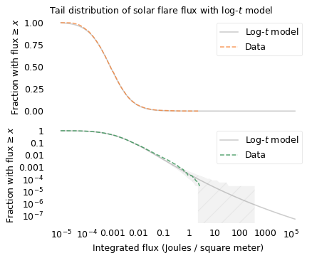
This example shows that the distribution of the size of solar flares is longer-tailed than a lognormal distribution, which suggests that the largest possible solar flares might be substantially larger than the ones we have seen so far.
If we use the model to extrapolate beyond the data – which is always an uncertain thing to do – we expect 2.4 flares per million to exceed 10 Joules per square meter, and 0.36 per million to exceed 100.
t_dist.sf([1, 2, 3], df, mu, sigma) * 1e6, 20e6 / n
(array([21.47023593, 2.41162628, 0.35574138]), 547.0459518599563)
t_dist.sf(5, df, mu, sigma) * 1e9, 1e9 / 36000
(array([14.61658962]), 27777.777777777777)
In the last 20 years we have observed about 36,000 flares, so it would take more than 500 years to observe a million. But in that time, we might see a solar flare 10 or 100 times bigger than the biggest we have seen so far.
Observations from the Kepler space telescope have found that a small fraction of stars like our Sun produce “superflares” up to 10,000 times bigger than the ones we have observed. At this point we don’t know whether these stars are different from our Sun in some way, or whether the Sun is also capable of producing superflares.
Lunar Craters#
While we have our eyes on the sky, let’s consider another source of potential disaster: an asteroid strike.
On March 11, 2022, an astronomer near Budapest, Hungary detected a new asteroid, now named 2022 EB5, on a collision course with Earth. Less than two hours later, it exploded in the atmosphere near Greenland. Fortunately, no large fragments reached the surface, and they caused no damage.
We have not always been so lucky. In 1908, a much larger asteroid entered the atmosphere over Siberia, causing an estimated 2 megaton explosion, about the same size as the largest thermonuclear device tested by the United States. The explosion flattened something like 80 million trees in an area covering 2100 square kilometers, almost the size of Rhode Island. Fortunately, the area was almost unpopulated; a similar-sized impact could destroy a large city.
These events suggest that we would be wise to understand the risks we face from large asteroids. To do that, we’ll look at evidence of damage they have done in the past: the impact craters on the Moon.
The largest crater on the near side of the moon, named Bailly, is 303 kilometers in diameter; the largest on the far side, the South Pole-Aitken basin, is roughly 2500 kilometers in diameter.
In addition to large, visible craters like these, there are innumerable smaller craters. The Lunar Crater Database catalogs nearly all of the ones larger than one kilometer, about 1.3 million in total. It is based on images taken by the Lunar Reconnaissance Orbiter, which NASA sent to the Moon in 2009.
# https://www.nytimes.com/2022/03/21/science/nasa-asteroid-strike.html

# https://en.wikipedia.org/wiki/Tunguska_event
# https://www.nasa.gov/centers/goddard/news/features/2010/biggest_crater.html
# https://en.wikipedia.org/wiki/Bailly_(crater)
# https://en.wikipedia.org/wiki/South_Pole%E2%80%93Aitken_basin
# https://astrogeology.usgs.gov/search/map/Moon/Research/Craters/lunar_crater_database_robbins_2018
# https://en.wikipedia.org/wiki/Lunar_Reconnaissance_Orbiter
# Robbins, S. J. (2018). A new global database of lunar impact craters >1–2 km: 1. Crater locations and sizes, comparisons with published databases, and global analysis. Journal of Geophysical Research: Planets, 124(4), pp. 871-892. https://doi.org/10.1029/2018JE005592
1740 * 2
3480
Download the data from https://astrogeology.usgs.gov/search/map/Moon/Research/Craters/lunar_crater_database_robbins_2018
# Looks like the old URL doesn't work
# download("https://pdsimage2.wr.usgs.gov/Individual_Investigations/moon_lro.kaguya_multi_craterdatabase_robbins_2018/data/lunar_crater_database_robbins_2018.csv")
!ls -lh lunar_crater_database_robbins_2018.csv
-rw-rw-r-- 1 downey downey 228M Mar 2 2023 lunar_crater_database_robbins_2018.csv
filename = "lunar_crater_database_robbins_2018.csv"
craters = pd.read_csv(filename, nrows=None)
craters.head()
| CRATER_ID | LAT_CIRC_IMG | LON_CIRC_IMG | LAT_ELLI_IMG | LON_ELLI_IMG | DIAM_CIRC_IMG | DIAM_CIRC_SD_IMG | DIAM_ELLI_MAJOR_IMG | DIAM_ELLI_MINOR_IMG | DIAM_ELLI_ECCEN_IMG | ... | DIAM_ELLI_ANGLE_IMG | LAT_ELLI_SD_IMG | LON_ELLI_SD_IMG | DIAM_ELLI_MAJOR_SD_IMG | DIAM_ELLI_MINOR_SD_IMG | DIAM_ELLI_ANGLE_SD_IMG | DIAM_ELLI_ECCEN_SD_IMG | DIAM_ELLI_ELLIP_SD_IMG | ARC_IMG | PTS_RIM_IMG | |
|---|---|---|---|---|---|---|---|---|---|---|---|---|---|---|---|---|---|---|---|---|---|
| 0 | 00-1-000000 | -19.83040 | 264.7570 | -19.89050 | 264.6650 | 940.960 | 21.31790 | 975.874 | 905.968 | 0.371666 | ... | 35.9919 | 0.007888 | 0.008424 | 0.636750 | 0.560417 | 0.373749 | 0.002085 | 0.000968 | 0.568712 | 8088 |
| 1 | 00-1-000001 | 44.77630 | 328.6020 | 44.40830 | 329.0460 | 249.840 | 5.99621 | 289.440 | 245.786 | 0.528111 | ... | 127.0030 | 0.011178 | 0.015101 | 1.052780 | 0.209035 | 0.357296 | 0.005100 | 0.004399 | 0.627328 | 2785 |
| 2 | 00-1-000002 | 57.08660 | 82.0995 | 56.90000 | 81.6464 | 599.778 | 21.57900 | 632.571 | 561.435 | 0.460721 | ... | 149.1620 | 0.008464 | 0.019515 | 0.776149 | 0.747352 | 0.374057 | 0.003095 | 0.002040 | 0.492373 | 5199 |
| 3 | 00-1-000003 | 1.96124 | 230.6220 | 1.95072 | 230.5880 | 558.762 | 14.18190 | 568.529 | 546.378 | 0.276416 | ... | 133.6910 | 0.007079 | 0.007839 | 0.526945 | 0.532872 | 1.262710 | 0.004496 | 0.001400 | 0.595221 | 4341 |
| 4 | 00-1-000004 | -49.14960 | 266.3470 | -49.18330 | 266.3530 | 654.332 | 17.50970 | 665.240 | 636.578 | 0.290365 | ... | 87.6468 | 0.008827 | 0.017733 | 0.568958 | 0.758631 | 1.383530 | 0.004626 | 0.001533 | 0.545924 | 5933 |
5 rows × 21 columns
diameters = craters["DIAM_CIRC_IMG"]
diameters.describe()
count    1.296796e+06
mean     2.436963e+00
std      5.519133e+00
min      1.000000e+00
25%      1.242710e+00
50%      1.606840e+00
75%      2.380860e+00
max      2.491870e+03
Name: DIAM_CIRC_IMG, dtype: float64
mags = np.log10(diameters)
mags.describe()
count    1.296796e+06
mean     2.730862e-01
std      2.483783e-01
min      0.000000e+00
25%      9.436979e-02
50%      2.059726e-01
75%      3.767339e-01
max      3.396525e+00
Name: DIAM_CIRC_IMG, dtype: float64
n = mags.count()
n
1296796
surv = make_surv(mags)
mu, sigma = fit_truncated_normal(surv)
[0.27308865 0.24837722]
[0.27308867 0.24837722]
[0.27308865 0.24837723]
[0.05295431 0.37367805]
[0.05295432 0.37367805]
[0.05295431 0.37367806]
[-0.25451594  0.46113896]
[-0.25451595  0.46113896]
[-0.25451594  0.46113898]
[-0.34244255  0.4572347 ]
[-0.34244256  0.4572347 ]
[-0.34244255  0.45723471]
[-0.2936525   0.44014652]
[-0.29365252  0.44014652]
[-0.2936525   0.44014653]
[-0.29545249  0.44042469]
[-0.2954525   0.44042469]
[-0.29545249  0.44042471]
[-0.29531495  0.44037601]
[-0.29531496  0.44037601]
[-0.29531495  0.44037602]
low, high = mags.min(), mags.max() * 0.99
qs = np.linspace(low, high, 2000)
surv_model = truncated_normal_sf(qs, mu, sigma)
xlabel = "Crater diameter (kilometers)"
ylabel = "Fraction with diameter ≥ $x$"
xlabels = [1, 3, 10, 100, 1000]
xticks = np.log10(xlabels)
yticks = [1, 0.1, 0.01, 1e-3, 1e-4, 1e-5, 1e-6, 1e-6]
ylabels = [1, 0.1, 0.01, 0.001, "$10^{-4}$", "$10^{-5}$", "$10^{-6}$", "$10^{-7}$"]
The following figure shows the distribution of these crater sizes, compared to a log-\(t\) model.
y1 * 1e6, y2 * 1e6
(218.81838074390188, 3.3991818848706328)
x = np.log10(1000)
surv(x), surv_model(x)
(array(3.08452525e-06), array(1.46578142e-13))
# 50 per sextillion

norm(mu, sigma).sf(high) * 1e18
49.38523077882056
df = minimize_df(10, surv, [(0, 20)])
mu, sigma = fit_truncated_t(df, surv)
df, mu, sigma
(array([11.13359356]), -0.2019431517012043, 0.37469477145698354)
low, high = surv.qs.min(), surv.qs.max()
qs = np.linspace(low, 1.2 * high, 2000)
surv_model2 = truncated_t_sf(qs, df, mu, sigma)
cutoff2 = surv_model2.qs <= 1.03 * high
model_label = "Log-$t$ model"
axs = plot_two(
    surv,
    surv_model2[cutoff2],
    n,
    hatch="/",
    title="Moon crater diameters with log-$t$ model",
)

plt.tight_layout()
savefig("longtail12.png")
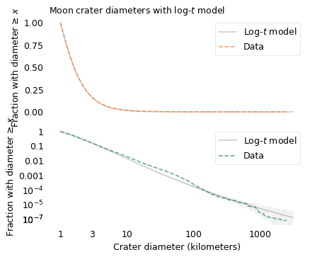
Since the dataset does not include craters smaller than one kilometer, I cut off the model at the same threshold. We can assume that there are many smaller craters, but with this dataset we can’t tell what the distribution of their sizes looks like.
The log-\(t\) model fits the distribution well, but it’s not perfect: there are more craters near 100 km than the model expects, and fewer craters larger than 1000 km. As usual, the world is under no obligation to follow simple rules, but this model does pretty well.
We might wonder why. To explain the distribution of crater sizes, it helps to think about where they come from. Most of the craters on the Moon were formed during a period in the life of the solar system called the “Late Heavy Bombardment”, about 4 billion years ago. During this period, an unusual number of asteroids were displaced from the asteroid belt – possibly by interactions with large outer planets – and some of them collided with the Moon.
Asteroids#
The Jet Propulsion Laboratory (JPL) and NASA provide data related to asteroids, comets and other small bodies in our solar system. From their Small-Body Database, I selected asteroids in the “main asteroid belt” between the orbits of Mars and Jupiter.
There are more than one million asteroids in this dataset, about 136,000 with known diameter. The largest are Ceres (940 kilometers in diameter), Vesta (525 km), Pallas (513 km), and Hygeia (407 km). The smallest are less than one kilometer.
I downloaded the data using the Small-Body Database
Selecting Inner, outer, and main belt asteroids
Variables: IAU name, diameter, GM (mass times gravitational constant G)
asteroids = pd.read_csv(filename, low_memory=False)
asteroids.shape
(1138975, 3)
Fans of The Expanse will recognize the names of the largest asteroids in the Belt.
asteroids.dropna().sort_values(by="diameter").tail()
| name | diameter | GM | |
|---|---|---|---|
| 693 | Interamnia | 306.313 | 5.000000 |
| 9 | Hygiea | 407.120 | 7.000000 |
| 1 | Pallas | 513.000 | 13.630000 |
| 3 | Vesta | 525.400 | 17.288245 |
| 0 | Ceres | 939.400 | 62.628400 |
asteroids.dropna().sort_values(by="diameter").head()
| name | diameter | GM | |
|---|---|---|---|
| 241 | Ida | 32.000 | 0.00275 |
| 251 | Mathilde | 52.800 | 0.00689 |
| 21 | Kalliope | 167.536 | 0.49100 |
| 106 | Camilla | 210.370 | 0.74750 |
| 15 | Psyche | 226.000 | 1.53000 |
asteroids["diameter"].describe()
count    135915.000000
mean          5.265815
std           8.495350
min           0.347000
25%           2.783000
50%           3.940000
75%           5.651000
max         939.400000
Name: diameter, dtype: float64
mags = np.log10(asteroids["diameter"])
mags.describe()
count    135915.000000
mean          0.613943
std           0.257474
min          -0.459671
25%           0.444513
50%           0.595496
75%           0.752125
max           2.972851
Name: diameter, dtype: float64
n = mags.count()
n
135915
surv = make_surv(mags)
mu, sigma = fit_truncated_normal(surv)
[0.61406612 0.2574008 ]
[0.61406614 0.2574008 ]
[0.61406612 0.25740082]
[0.59649365 0.22729091]
[0.59649367 0.22729091]
[0.59649365 0.22729093]
[0.59765045 0.22862602]
[0.59765047 0.22862602]
[0.59765045 0.22862603]
[0.59766666 0.22865271]
[0.59766668 0.22865271]
[0.59766666 0.22865273]
from utils import truncated_normal_pmf

low, high = mags.min(), mags.max() * 0.99
qs = np.linspace(low, high, 2000)
pmf_model = truncated_normal_pmf(qs, mu, sigma)
surv_model = pmf_model.make_surv()
xlabel = "Asteroid diameter (kilometers)"
ylabel = "Fraction with diameter ≥ $x$"
xticks = [0, 1, 2, 3]
xlabels = [1, 10, 100, 1000]
x = 1.5
y1 = surv(x)
y2 = surv_model(x)
y1 * 1e6, y2 * 1e6
(8188.941617943904, 39.34458611676295)
cutoff = surv_model > 1e-6
yticks = [1, 0.1, 0.01, 1e-3, 1e-4, 1e-5, 1e-6]
ylabels = [1, 0.1, 0.01, "$10^{-3}$", "$10^{-4}$", "$10^{-5}$", "$10^{-6}$"]
model_label = "Lognormal model"
axs = plot_two(
    surv,
    surv_model[cutoff],
    n,
    title="Tail distribution of asteroid diameters with lognormal model",
)
plt.tight_layout()
savefig("longtail13.png")
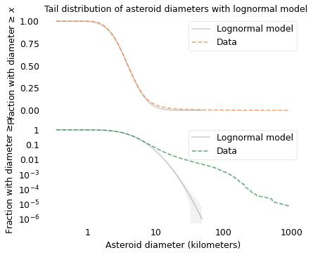
The following figure shows the distribution of asteroid sizes compared to a log-\(t\) model.
df = minimize_df(10, surv, [(0, 20)])
df = 6.5
mu, sigma = fit_truncated_t(df, surv)
df, mu, sigma
(6.5, 0.5953882516804466, 0.2150180564203059)
low, high = surv.qs.min(), surv.qs.max()
qs = np.linspace(low, 1.0 * high, 2000)
surv_model2 = truncated_t_sf(qs, df, mu, sigma)
cutoff2 = surv_model2.qs <= 1.0 * high
model_label = "Log-$t$ model"
axs = plot_two(
    surv,
    surv_model2[cutoff2],
    n,
    hatch="/",
    title="Tail distribution of asteroid diameters with log-$t$ model",
)
plt.tight_layout()
savefig("longtail14.png")
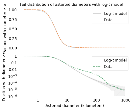
In the top figure, we see that the log-\(t\) model fits the data well in the middle of the range, except possibly near 1 kilometer. In the bottom, we see that the log-\(t\) model does not fit the tail of the distribution particularly well: there are more asteroids near 100 km than the model predicts. So the distribution of asteroid sizes does not strictly follow a log-\(t\) distribution. Nevertheless, we can use it to explain the distribution of crater sizes, as I’ll show in the next section.
Origins of Long-Tailed Distributions#
One of the reasons long-tailed distributions are common in natural systems is that they are persistent; for example, if a quantity comes from a long-tailed distribution and you multiply it by a constant or raise it to a power, the result follows a long-tailed distribution.
Long-tailed distributions also persist when they interact with other distributions. When you add together two quantities, if either comes from a long-tailed distribution, the sum follows a long-tailed distribution, regardless of what the other distribution looks like. Similarly, when you multiply two quantities, if either comes from a long-tailed distribution, the product usually follows a long-tailed distribution. This property might explain why the distribution of crater sizes is long-tailed.
Empirically – that is, based on data rather than a physical model – the diameter of an impact crater depends on the diameter of the projectile that created it, raised to the power 0.78, and on the impact velocity raised to the power 0.44. It also depends on the density of the asteroid and the angle of impact.
Source: Melosh, Planetary Surface Processes.
As a simple model of this relationship, I’ll simulate the crater formation process by drawing asteroid diameters from the distribution in the previous section and drawing the other factors – density, velocity, and angle – from a lognormal distribution with parameters chosen to match the data. The following figure shows the results from this simulation along with the actual distribution of crater sizes.
diam_asteroid = asteroids["diameter"].dropna()
diam_crater = craters["DIAM_CIRC_IMG"].dropna()
diam_asteroid.count(), diam_crater.count()
(135915, 1296796)
surv_crater = make_surv(np.log10(diam_crater))
np.random.seed(17)
n = diam_crater.count()
resample_asteroid = diam_asteroid.sample(100 * n, replace=True)
# resample_asteroid = diam_asteroid
rvs = np.random.normal(size=resample_asteroid.count())
len(rvs)
129679600
def error_func_pred(params):
    """Error function for finding parameters for the asteroid problem.

    params: tuple of mu and sigma

    returns: array of differences in the survival functions
    """
    mu, sigma = params
    factors = np.power(10, rvs * sigma + mu)
    pred_crater = factors * resample_asteroid**0.78
    mags = np.log10(pred_crater)
    cutoff = mags >= surv_crater.qs.min()
    surv_pred = make_surv(mags[cutoff])

    ps = np.logspace(-1, -5, 20)
    qs = surv.inverse(ps)

    error = surv_crater(qs) - surv_pred(qs)
    return error
mu = -3.194
sigma = 0.883
params = mu, sigma
error_func_pred(params)
array([-3.16249439e-04, -2.73415007e-05,  1.20415497e-04,  2.96512650e-04,
        4.48439739e-04,  6.12564529e-04,  4.29226980e-04,  2.16708737e-04,
        1.21459936e-04,  6.07299681e-05,  3.32894198e-05,  2.09586479e-05,
        8.46778641e-06,  8.78063634e-06,  7.08561326e-06,  1.45431455e-07,
        1.04829884e-05,  1.38803636e-05,  1.38803636e-05,  4.62678787e-06])
from scipy.optimize import least_squares

def run_minimize():
    """Find the values of mu and sigma that solve the asteroid problem.
    """
    res = least_squares(error_func_pred, x0=params, xtol=1e-3, diff_step=0.01)
    assert res.success
    mu, sigma = res.x
    return mu, sigma


# mu, sigma = run_minimize()
factors = np.power(10, rvs * sigma + mu)
pred_crater = factors * resample_asteroid**0.78
mags = np.log10(pred_crater)
cutoff = mags >= surv_crater.qs.min()
surv_pred = make_surv(mags[cutoff])
surv_pred.head()
| probs | |
|---|---|
| diameter | |
| 0.000001 | 1.000000 |
| 0.000002 | 0.999995 |
| 0.000005 | 0.999990 |
xlabel = "Crater diameter (kilometers)"
ylabel = "Fraction with diameter ≥ $x$"

xticks = [0, 1, 2, 3]
xlabels = [1, 10, 100, 1000]

cutoff = surv_pred.qs >= 0
model_label = "Simulated crater sizes"

axs = plot_two(
    surv_crater,
    surv_pred,
    n,
    hatch="/",
    title="Moon crater diameters with simulation results",
)

plt.tight_layout()
savefig("longtail15.png")
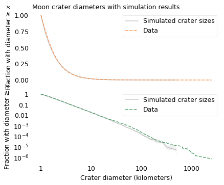
The simulation results are a good match for the data. This example suggests that the distribution of crater sizes can be explained by the relationship between the distributions of asteroid sizes and other factors like velocity and density.
In The Fractal Geometry of Nature, Benoit Mandelbrot proposes what he calls a “heretical” explanation for the prevalence of long-tailed distributions in natural systems: there may be only a few systems that generate long-tailed distributions, but interactions between systems might cause them to propagate.
He suggests that data we observe are often “the joint effect of a fixed underlying true distribution and a highly variable filter”, and “a wide variety of filters leave their asymptotic behavior unchanged”.
The long tail in the distribution of asteroid sizes is an example of “asymptotic behavior”. And the relationship between the size of an asteroid and the size of the crater it makes is an example of a “filter”. In this relationship, the size of the asteroid gets raised to a power and multiplied by a “highly-variable” lognormal distribution. These operations change the location and spread of the distribution, but they don’t change the shape of the tail.
When Mandelbrot wrote in the 1970s, this explanation might have been heretical, but now long-tailed distributions are more widely known and better understood. What was heresy then is orthodoxy now.
Stock Market Crashes#
Natural disasters cost lives and destroy property. By comparison, stock market crashes might seem less frightening, but while they don’t cause fatalities, they can destroy more wealth, more quickly. For example, the stock market crash on October 19, 1987, known as Black Monday, caused total worldwide losses of $1.7 trillion. The amount of wealth that disappeared in one day, at least on paper, exceeded the total cost of every earthquake in the 20th century and so far in the 21st.
Like natural disasters, the distribution of magnitudes of stock market crashes is long-tailed. To demonstrate, I’ll use data from the MeasuringWorth Foundation which has compiled the value of the Dow Jones Industrial Average at the end of each day from February 16, 1885 to the present, with adjustments at several points to make the values consistent. The series I collected ends on May 6, 2022, so it includes 37,512 days.
# "Citation: Samuel H. Williamson, 'Daily Closing Value of the Dow Jones Average, 1885 to Present,' MeasuringWorth, 2022. "

# https://www.measuringworth.com/datasets/DJA
djia = pd.read_csv(filename, skiprows=4)
djia.shape
(37512, 2)
djia.head()
| Date | DJIA | |
|---|---|---|
| 0 | 2/16/1885 | 30.9226 |
| 1 | 2/17/1885 | 31.3365 |
| 2 | 2/18/1885 | 31.4744 |
| 3 | 2/19/1885 | 31.6765 |
| 4 | 2/20/1885 | 31.4252 |
djia.tail()
| Date | DJIA | |
|---|---|---|
| 37507 | 5/2/2022 | 33061.50 |
| 37508 | 5/3/2022 | 33128.79 |
| 37509 | 5/4/2022 | 34061.06 |
| 37510 | 5/5/2022 | 32997.97 |
| 37511 | 5/6/2022 | 32899.37 |
In percentage terms, the largest single-day drop was 22.6%, during the Black Monday crash. The second largest drop was 12.9% on March 16, 2020, during the crash caused by the COVID-19 pandemic. Numbers three and four on the list were 12.8% and 11.7%, on consecutive days during Wall Street Crash of 1929.
diff = np.log10(djia["DJIA"]).diff()
djia["change"] = (10**diff - 1) * 100
djia.sort_values(by="change").head()
| Date | DJIA | change | |
|---|---|---|---|
| 28833 | 10/19/1987 | 1738.74 | -22.610538 |
| 36978 | 3/16/2020 | 20188.52 | -12.926547 |
| 13297 | 10/28/1929 | 260.64 | -12.820684 |
| 13298 | 10/29/1929 | 230.07 | -11.728821 |
| 36976 | 3/12/2020 | 21200.62 | -9.988443 |
On the positive side, the largest single-day gain was on March 15, 1933, when the index gained 15.3%. There were other large gains in October 1929 and October 1931. The largest gain of the 21st century, so far, was on March 24, 2020, when the index gained 11.4% in expectation that the U.S. Congress would pass a large economic stimulus bill.
djia.sort_values(by="change").tail()
| Date | DJIA | change | |
|---|---|---|---|
| 36984 | 3/24/2020 | 20704.9100 | 11.365038 |
| 13299 | 10/30/1929 | 258.4700 | 12.344069 |
| 13871 | 10/6/1931 | 99.3400 | 14.870490 |
| 14292 | 3/15/1933 | 62.1000 | 15.341753 |
| 0 | 2/16/1885 | 30.9226 | NaN |
But these large moves are unusual; on 95% of days, the change is less than 2 percentage points either way.
djia["change"].abs().describe()
count    37511.000000
mean         0.712317
std          0.799769
min          0.000000
25%          0.217753
50%          0.493605
75%          0.935523
max         22.610538
Name: change, dtype: float64
(djia["change"].abs() < 2).mean()
0.9453508210705908
(djia["change"] < -2).mean()
0.028897419492429088
all_mags = np.log10(djia["DJIA"]).diff()
all_mags.describe()
count    37511.000000
mean         0.000081
std          0.004660
min         -0.111318
25%         -0.001970
50%          0.000195
75%          0.002291
max          0.061987
Name: DJIA, dtype: float64
(all_mags > 0).mean(), (all_mags < 0).mean(), (all_mags == 0).mean()
(0.5231392621027938, 0.4713158455960759, 0.005518234165067178)
r = 10 ** all_mags.mean()
(r - 1) * 100
0.018582199949923606
As an aside, the index climbed on 52.3% of days, fell on 47.1% of days, and closed exactly where it opened on the remaining 0.06% of days. The average increase was only 0.02% per day, but with about 250 trading days per year, that amounts to an increase of 4.8% annually. After 37,512 days, the total increase is more than 100,000%. So that’s a pretty good return on investment, if you made the investment in 1885.
r**250 - 1
0.04754694096007417
n = len(all_mags)
n, r**n - 1
(37512, 1063.1240848647278)
start, end = djia["DJIA"].iloc[[0, -1]]
start, end, end / start - 1
(30.9226, 32899.37, 1062.926383939255)
losses = all_mags < 0
losses.mean()
0.4713158455960759
mags = -all_mags[losses]
mags.describe()
count    1.768000e+04
mean     3.196865e-03
std      3.704198e-03
min      7.287896e-07
25%      9.450282e-04
50%      2.151678e-03
75%      4.170744e-03
max      1.113182e-01
Name: DJIA, dtype: float64
10 ** (-mags.max())
0.7738946206503647
n = mags.count()
n
17680
surv = make_surv(mags)
mu, sigma = fit_truncated_normal(surv)
mu, sigma
[0.00319705 0.00370412]
[0.00319706 0.00370412]
[0.00319705 0.00370414]
[-0.0013507   0.00550956]
[-0.00135072  0.00550956]
[-0.0013507   0.00550957]
[-0.00621391  0.00604884]
[-0.00621392  0.00604884]
[-0.00621391  0.00604886]
[-0.01126   0.007184]
[-0.01126002  0.007184  ]
[-0.01126     0.00718402]
[-0.01332923  0.00747085]
[-0.01332924  0.00747085]
[-0.01332923  0.00747086]
[-0.01298826  0.00737537]
[-0.01298827  0.00737537]
[-0.01298826  0.00737538]
[-0.01293662  0.00736386]
[-0.01293664  0.00736386]
[-0.01293662  0.00736387]
[-0.01293473  0.00736343]
[-0.01293475  0.00736343]
[-0.01293473  0.00736344]
(-0.012934732189136055, 0.007363429563516698)
low, high = surv.qs.min(), surv.qs.max()
qs = np.linspace(low, high, 2000)
surv_model = truncated_normal_sf(qs, mu, sigma)
xlabel = "One day percent change"
xlabels = ["no change", "-5%", "-10%", "-15%", "-20%"]
xticks = -np.log10([1, 0.95, 0.9, 0.85, 0.8])
xticks
array([-0. , 0.02227639, 0.04575749, 0.07058107, 0.09691001])
surv(xticks)[1] * 100
0.48076923076922906
cutoff = surv_model > 1e-5
yticks = [1, 0.1, 0.01, 1e-3, 1e-4, 1e-5]
ylabels = [1, 0.1, 0.01, 0.001, "$10^{-4}$", "$10^{-5}$"]
Since we are interested in stock market crashes, I selected the 17,680 days when the value of the index dropped.
model_label = "Lognormal model"
ylabel = "Fraction with drop ≥ $x$"

axs = plot_two(
    surv,
    surv_model[cutoff],
    n,
    title="Tail distribution of negative changes with lognormal model",
)

plt.tight_layout()
savefig("longtail16.png")
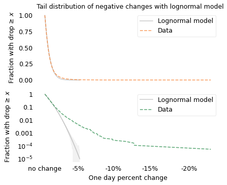
On the left, the lognormal model seems to fit the distribution well, but again there are big differences hiding in the tail. On the right, we can see that the lognormal model does not fit the tail of the distribution at all.
The following figure shows the distribution of these negative percentage changes compared to a log-\(t\) model.
df = minimize_df(3, surv, [(1, 20)])
mu, sigma = fit_truncated_t(df, surv)
df, mu, sigma
(array([3.8945931]), -0.002607418984953457, 0.003426713548607919)
low, high = surv.qs.min(), surv.qs.max()
qs = np.linspace(low, 1.02 * high, 2000)
surv_model = truncated_t_sf(qs, df, mu, sigma)
cutoff = surv_model.qs <= high
model_label = "Log-$t$ model"
axs = plot_two(
    surv,
    surv_model,
    n,
    hatch="/",
    title="Tail distribution of stock market changes with log-$t$ model",
)
surv.iloc[-2:].plot(color="C0", style="o")

plt.tight_layout()
savefig("longtail17.png")
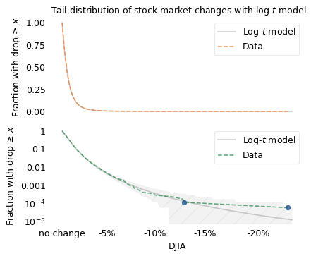
The top figure shows that the log-\(t\) model fits the left side of the distribution well. The bottom figure shows that it fits the tail well, with the possible exception of the last data point, the 1987 crash, which falls just at the edge of variation we expect. According to the model, there is only a 5% chance that we would see a crash as big as this one after 17,680 down days.
x = surv.qs.max()
y1 = surv(x)
y2 = surv_model(x)
n, y1, y2, y1 / y2
(17680, array(5.6561086e-05), array(1.28916302e-05), 4.387426949065176)
1 - t_dist(df, mu, sigma).cdf(x) ** n
array([0.0542351])
There are two interpretations of this observation: maybe Black Monday was a deviation from the model, or maybe we were just unlucky. These possibilities are the topic of some controversy, as I’ll discuss in the next section.
Black and Gray Swans#
If you have read The Black Swan, by Nassim Taleb, the examples in this chapter provide context for understanding black swans and their relatives, gray swans.
In Taleb’s vocabulary, a black swan is a large, impactful event that was considered extremely unlikely before it happened, based on a model of prior events. If the distribution of event sizes is actually long-tailed and the model is Gaussian, black swans will happen with some regularity.
For example, if we use a Gaussian distribution to model the magnitudes of earthquakes, we predict that the probability of a magnitude 7 earthquake is about 4 per sextillion (\(10^{18}\)). The actual rate in the dataset we looked at is about 6 per million, which is more likely by a factor of a trillion (\(10^{12}\)). When a magnitude 7 earthquake occurs, it would be a black swan if your predictions were based on the Gaussian model.
# x = 7
# surv(x)*1e6, surv_model(x)*1e18

# 6.318484473557436, 4.618502751454663
However, black swans can be “tamed” by using appropriate long-tailed distributions, as we did in this chapter. According to the log-\(t\) model, based on the distribution of past earthquakes, and the UCERF3 model, which is based on geological physics in addition to data, we expect a magnitude 7 quake to occur once every few decades, on average. To someone whose predictions are based on these models, such an earthquake would not be particularly surprising. In Taleb’s vocabulary, it would be a gray swan: large and impactful, but not unexpected.
This part of Taleb’s thesis is uncontroversial: if you use a model that does not fit the data, your predictions will probably fail. In this chapter, we’ve seen several examples that demonstrate this point.
However, Taleb goes farther, asserting that long-tailed distributions “account for a few black swans, but not all.” He explains, “A gray swan concerns modelable extreme events, a black swan is about unknown unknowns.”
A superflare might be an example of an untamed black swan. As I mentioned in the section on solar flares, we have observed superflares on other stars that are 10,000 bigger than the biggest flare we have seen from the Sun, so far.
According to the log-\(t\) model, the probability of a flare that size is a few per billion, which means we should expect one every 30,000 years, on average. But that estimate extrapolates beyond the data by four powers of 10; we have little confidence that the model is valid in that range. Maybe the processes that generate superflares are different from the processes that generate normal flares, and they are actually more likely than the model predicts. Or maybe our Sun is different from stars that produce superflares, and it will never produce a superflare, ever. A model based on 20 years of data can’t distinguish among these possibilities; they are unknown unknowns.
The difference between black and gray swans is the state of our knowledge and our best models. If a superflare happened tomorrow, it would be a black swan. But as we learn more about the Sun and other stars, we might create better models that predict large solar flares with credible accuracy. In the future, a superflare might be a gray swan.
However, predicting rare events will always be difficult, and there may always be black swans.
In a Long-Tailed World#
In fact, there are two reasons we will always have a hard time dealing with rare, large events. First, they are rare, and people are bad at comprehending small probabilities. Second, they are large, and people are bad at comprehending very large magnitudes.
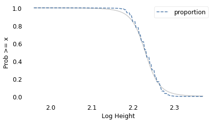
To demonstrate the second point, let’s imagine a world where the distribution of human height is not Gaussian or even lognormal; instead, it follows a long-tailed distribution like the various disasters in this chapter. Specifically, suppose it follows a log-\(t\) distribution with the same tail thickness as the distribution of disaster costs, but with the same mean as the distribution of human height.
If you woke up in this Long-Tailed World, you might not notice the difference immediately. The first few people you meet would probably be of unsurprising height.
brfss = pd.read_hdf(filename, "brfss")
height = brfss["HTM4"]
height.quantile([0.25, 0.75])
0.25    163.0
0.75    178.0
Name: HTM4, dtype: float64
mags = np.log10(height)
n = mags.count()
mags.describe()
count    375271.000000
mean          2.229956
std           0.028219
min           1.959041
25%           2.212188
50%           2.230449
75%           2.250420
max           2.369216
Name: HTM4, dtype: float64
surv = make_surv(mags)
df = minimize_df(5, surv, [(1, 1e6)])
df
array([999859.46341698])
df = 3.53  # same as distribution of disasters
mu, sigma = fit_truncated_t(df, surv)
df, mu, sigma
(3.53, 2.2293001672048596, 0.025915097488203958)
low, high = surv.qs.min(), surv.qs.max()
qs = np.linspace(low, high, 2000)
surv_model = truncated_t_sf(qs, df, mu, sigma)
model_label = "Log-$t$ model"
xlabel = ""
ylabel = ""
xticks = []
xlabels = xticks
axs = plot_two(surv, surv_model, n)
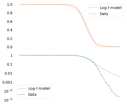
surv_model.plot(color="gray", alpha=0.4)
surv.plot(ls="--")
decorate(xlabel="Log Height", ylabel="Prob >= x")
dist = t_dist(df, mu, sigma)
ps = [0.9, 0.99, 0.999, 1 - 1 / 10000, 1 - 1e-6, 1 - 1 / 330e6, 1 - 1 / 7e9]
ps
[0.9, 0.99, 0.999, 0.9999, 0.999999, 0.999999996969697, 0.9999999998571428]
(height >= 277).mean() * 7e9
0.0
Out of 100 people, the tallest might be 215 cm.
If you see 1000 people, the tallest of them might be 277 cm.
Out of 10,000 people, the tallest would be more than 4 meters tall.
Out of a million people in Long-tailed World, the tallest would be 59 meters . In a country the size of the United States, the tallest person would be 160,000 kilometers tall.
And in a world population of 7 billion, the tallest would be 14 quintillion kilometers tall, which is about 1500 light years, almost three times the distance from our Sun to Betelgeuse.
This example shows how long-tailed distributions violate our intuition and strain our imagination. Most of the things we observe directly in the world follow Gaussian and lognormal distributions. The things that follow long-tailed distributions are hard to perceive, which makes them hard to conceive.
However, by collecting data and using appropriate tools to understand it, we can make better predictions and – I hope – prepare accordingly. Otherwise, rare events will continue to take us by surprise and catch us unprepared.
In this chapter I made it a point to identify the sources of the data I used; I am grateful to the following agencies and organizations for making this data freely available:
The Space Weather Prediction Center and the National Centers for Environmental Information, funded by the National Oceanic and Atmospheric Administration (NOAA),
The Southern California Earthquake Data Center, funded by the U.S. Geological Survey (USGS),
The Moon Crater Database, provided by the USGS using data collected by NASA,
The JPL Small Body Database, provided by the Jet Propulsion Laboratory and funded by NASA,
The history of the Dow Jones Industrial Average, provided by the MeasuringWorth Foundation, a non-profit organization with the mission to make available “the highest quality and most reliable historical data on important economic aggregates”.
Collecting data like this requires satellites, space probes, seismometers, and other instruments; and processing it requires time, expertise, and other resources. These activities are expensive, but if we use the data to predict, prepare for, and mitigate the costs of disaster, it will pay for itself many times over.