Chile Earthquake Magnitudes

Exploring the distribution of earthquake magnitudes in Chile using the relocated catalogue from the Centro Sismológico Nacional (CSN), 1982–mid-2020.

Potin et al. (2024), doi:10.1785/0220240047

# Install empiricaldist if we don't already have it

try:
    import empiricaldist
except ImportError:
    !pip install empiricaldist

from os.path import basename, exists


def download(url):
    filename = basename(url)
    if not exists(filename):
        from urllib.request import urlretrieve

        local, _ = urlretrieve(url, filename)
        print("Downloaded " + local)


download(
    "https://github.com/AllenDowney/ProbablyOverthinkingIt/raw/book/notebooks/utils.py"
)

import pandas as pd
import numpy as np
import matplotlib.pyplot as plt

from empiricaldist import Cdf, Surv
from utils import decorate, set_pyplot_params, make_surv, plot_error_bounds

set_pyplot_params()

Load the catalogue

Data from Potin et al. (2024): a revised, relocated Chilean seismic catalogue covering 1982 to mid-2020. See chile/chilean_seismic_catalogue-1982-2020-publication_release/README.md for column definitions and citation details.

DATA_DIR = "chile/chilean_seismic_catalogue-1982-2020-publication_release"
SEISMICITY_PATH = f"{DATA_DIR}/CHILE_SEISMICITY_RELOCATED.csv"

data = pd.read_csv(SEISMICITY_PATH)
data["magnitude_type"] = data["magnitude_type"].str.strip()
data.shape

(118004, 13)

data.head()

	#	year	month	day	hour	minute	seconds	longitude	latitude	depth	rms	magnitude	magnitude_type
0	0	1982	1	8	0	32	52.05	-71.760237	-32.218361	11.7341	0.95	NaN	xx
1	1	1982	1	9	1	6	18.81	-73.147276	-33.919849	5.3619	0.86	NaN	xx
2	2	1982	1	9	20	28	47.24	-70.053573	-32.952820	118.5877	0.27	NaN	xx
3	3	1982	1	12	15	4	33.20	-70.431024	-32.467427	89.8999	0.08	NaN	xx
4	4	1982	1	13	11	20	3.02	-69.627611	-31.559731	46.6019	1.49	NaN	xx

data.describe(include="all")

	#	year	month	day	hour	minute	seconds	longitude	latitude	depth	rms	magnitude	magnitude_type
count	118004.00000	118004.000000	118004.000000	118004.000000	118004.000000	118004.000000	118004.000000	118004.000000	118004.000000	118004.000000	118004.000000	109310.000000	118004
unique	NaN	NaN	NaN	NaN	NaN	NaN	NaN	NaN	NaN	NaN	NaN	NaN	7
top	NaN	NaN	NaN	NaN	NaN	NaN	NaN	NaN	NaN	NaN	NaN	NaN	l
freq	NaN	NaN	NaN	NaN	NaN	NaN	NaN	NaN	NaN	NaN	NaN	NaN	89168
mean	59001.50000	2008.268915	6.537863	15.628521	11.320065	29.394961	30.028944	-70.540887	-29.325809	68.141672	0.357229	3.177608	NaN
std	34064.96492	9.381915	3.453024	8.782564	6.920552	17.304747	17.315109	1.531607	5.681583	56.104951	0.195222	0.792424	NaN
min	0.00000	1982.000000	1.000000	1.000000	0.000000	0.000000	0.000000	-76.229448	-45.979579	-4.954000	0.010000	0.200000	NaN
25%	29500.75000	2003.000000	4.000000	8.000000	5.000000	14.000000	15.050000	-71.741079	-33.416475	22.039650	0.230000	2.700000	NaN
50%	59001.50000	2010.000000	6.000000	16.000000	11.000000	29.000000	30.070000	-70.707791	-31.664178	52.116300	0.310000	3.100000	NaN
75%	88502.25000	2016.000000	10.000000	23.000000	17.000000	44.000000	45.010000	-69.277223	-23.024681	105.557100	0.440000	3.600000	NaN
max	118003.00000	2020.000000	12.000000	31.000000	23.000000	59.000000	59.990000	-64.810972	-17.817892	336.550300	2.430000	8.800000	NaN

Magnitude is reported on several scales (l local, c coda, w and ww moment magnitude). Many early events have no magnitude estimate.

data["magnitude_type"].value_counts()

magnitude_type
l     89168
c     18629
xx     8694
ww     1238
W       265
B         9
          1
Name: count, dtype: int64

no_mag = data["magnitude"].isna() | (data["magnitude_type"] == "xx")
no_mag.mean()

0.0736754686281821

Keep events with a valid magnitude for the distribution analysis.

events = data.loc[~no_mag].copy()
events.groupby("magnitude_type")["magnitude"].describe()

	count	mean	std	min	25%	50%	75%	max
magnitude_type
	1.0	4.000000	NaN	4.0	4.0	4.0	4.0	4.0
B	9.0	4.811111	0.329562	4.4	4.6	4.8	5.1	5.3
W	265.0	5.167170	1.093272	2.1	4.7	5.2	5.8	8.8
c	18629.0	3.108449	1.172345	0.2	2.8	3.5	3.8	6.4
l	89168.0	3.163719	0.653422	0.6	2.7	3.1	3.5	6.8
ww	1238.0	4.780210	0.484259	3.1	4.5	4.7	5.0	7.6

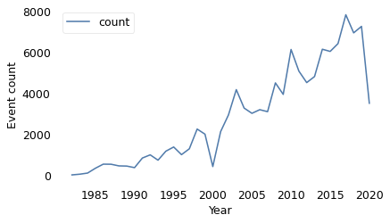
The number of events per year has been increasing, which suggests better detection.

events["year"].value_counts().sort_index().plot()
decorate(xlabel="Year", ylabel="Event count")

for mtype, group in events.groupby("magnitude_type"):
    Cdf.from_seq(group["magnitude"]).plot(label=mtype)

decorate(xlabel="Magnitude", ylabel="CDF")
plt.legend()
plt.savefig("chile_eda_cdf.png", dpi=300)

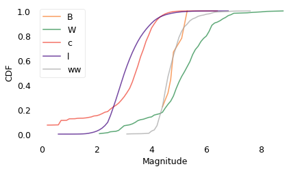
The distributions for the different kinds of magnitudes are substantially different. I’m not sure it’s valid to combine them, but for a first pass analysis, that’s what I’m going to do.

mags = events["magnitude"]
mags.describe()

count    109310.000000
mean          3.177608
std           0.792424
min           0.200000
25%           2.700000
50%           3.100000
75%           3.600000
max           8.800000
Name: magnitude, dtype: float64

As expected, there are only a few very large magnitudes.

(mags >= 7).sum(), (mags >= 7.5).sum(), mags.max()

(11, 6, 8.8)

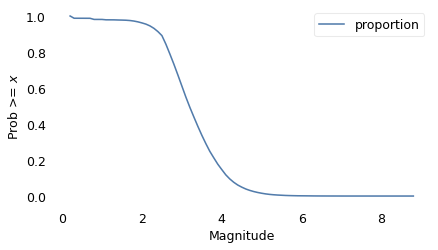
Here’s the tail distribution (fraction of values >= x for all x).

surv = make_surv(mags)

xlabel = "Magnitude"
ylabel = "Prob >= $x$"

surv.plot()

decorate(xlabel=xlabel, ylabel=ylabel)

Fit a Student t

Find the df parameter that best matches the tail, then the mu and sigma parameters that best match the percentiles.

from scipy.stats import t as t_dist


def truncated_t_sf(qs, df, mu, sigma):
    ps = t_dist.sf(qs, df, mu, sigma)
    surv_model = Surv(ps / ps[0], qs)
    return surv_model

from scipy.optimize import least_squares


def fit_truncated_t(df, surv):
    """Given df, find the best values of mu and sigma."""
    low, high = surv.qs.min(), surv.qs.max()
    qs_model = np.linspace(low, high, 1000)

    # match 20 percentiles from 10th to 99th
    ps = np.linspace(0.10, 0.9, 20)
    qs = surv.inverse(ps)

    def error_func_t(params, df, surv):
        mu, sigma = params
        surv_model = truncated_t_sf(qs_model, df, mu, sigma)

        error = surv(qs) - surv_model(qs)
        return error

    params = surv.mean(), surv.std()
    res = least_squares(error_func_t, x0=params, args=(df, surv), xtol=1e-3)
    assert res.success
    return res.x

from scipy.optimize import minimize


def minimize_df(df0, surv, bounds=[(1, 1e6)], ps=None):
    low, high = surv.qs.min(), surv.qs.max()
    qs_model = np.linspace(low, high * 1.0, 2000)

    if ps is None:
        t = surv.ps[0], surv.ps[-2]
        t = 0.1, surv.ps[-2]
        low, high = np.log10(t)
        ps = np.logspace(low, high, 30, endpoint=False)

    qs = surv.inverse(ps)

    def error_func_tail(params):
        (df,) = params
        mu, sigma = fit_truncated_t(df, surv)
        surv_model = truncated_t_sf(qs_model, df, mu, sigma)

        errors = np.log10(surv(qs)) - np.log10(surv_model(qs))
        return np.sum(errors**2)

    params = (df0,)
    res = minimize(error_func_tail, x0=params, bounds=bounds, tol=1e-3, method="Powell")
    assert res.success
    return res.x

Search for the value of df that best matches the tail behavior.

df = minimize_df(5, surv, [(1, 1000)])
df

array([8.92478953])

Given that value of df, find mu and sigma to best match percentiles.

mu, sigma = fit_truncated_t(df, surv)
df, mu, sigma

(array([8.92478953]), 3.209750270962042, 0.65453719080302)

Run the model out to magnitude 9.5

low, high = surv.qs.min(), 9.5
qs = np.linspace(low, high, 2000)
surv_model = truncated_t_sf(qs, df, mu, sigma)

On a linear scale:

model_label = "$t$ model"

surv_model.plot(color="gray", alpha=0.4, label=model_label)
surv.plot(color="C1", ls="--", label="Data")

decorate(xlabel=xlabel, ylabel=ylabel)
plt.savefig("chile3.png", dpi=300)

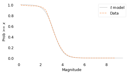
The model fits the data well above magnitude 3.

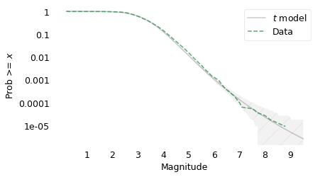
Now on a log-y scale:

yticks = [1, 0.1, 0.01, 1e-3, 1e-4, 1e-5]
ylabels = yticks
xticks = np.arange(1, 10)
xlabels = xticks

surv_model.plot(color="gray", alpha=0.4, label=model_label)
plot_error_bounds(Surv(surv_model), mags.count(), color="gray", hatch="/")
surv.plot(color="C2", ls="--", label="Data")

decorate(xlabel=xlabel, ylabel=ylabel, yscale="log")
plt.xticks(xticks, xlabels)
plt.yticks(yticks, ylabels)
plt.savefig("chile4.png", dpi=300)

And both together

def plot_two(surv, surv_model, n, hatch=None, title=""):
    """Plots tail distributions on linear-y and log-y scales.

    Uses global variables model_label, ylabel, xlabel, xticks, yticks, xlabels, ylabels.
    """
    fig, axs = plt.subplots(2, 1, figsize=(6, 5), sharex=True)

    plt.sca(axs[0])
    surv_model.plot(color="gray", alpha=0.4, label=model_label)
    if n < 1000:
        plot_error_bounds(Surv(surv_model), n, color="gray")
    surv.plot(color="C1", ls="--", label="Data")
    decorate(ylabel=ylabel, title=title)

    plt.sca(axs[1])
    surv_model.plot(color="gray", alpha=0.4, label=model_label)
    plot_error_bounds(Surv(surv_model), n, color="gray", hatch=hatch)
    surv.plot(color="C2", ls="--", label="Data")
    decorate(xlabel=xlabel, ylabel=ylabel, yscale="log")
    plt.xticks(xticks, xlabels)
    plt.yticks(yticks, ylabels)

    plt.tight_layout()
    return axs

plot_two(surv, surv_model, mags.count(), hatch="/")
plt.savefig("chile_t_model.png", dpi=300)

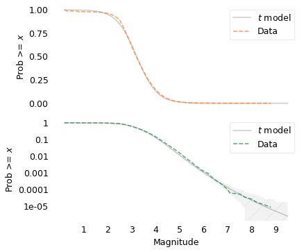
The model fits the tail behavior well and makes plausible predictions for very large earthquakes.

Copyright 2026 Allen B. Downey

Example related to Chapter 9 from Probably Overthinking It.

License: Attribution-NonCommercial-ShareAlike 4.0 International (CC BY-NC-SA 4.0)