Measuring the Overton Window

Measuring the Overton Window#

Chapter 12 of Probably Overthinking It is about changes in conservative beliefs over time and between cohorts.

While working on that chapter, I used a bit of Bayesian inference that is too technical to explain in the book. So I’ll explain it here.

Click here to run this notebook on Colab

Imports and Function Definitions#

Read the Data#

The HDF file contains three resamplings of the GSS data, with the keys gss0, gss1, and gss2. The resampled data correct for stratified sampling in the GSS survey design, and provide a coarse estimate of variability due to random sampling. I do development and testing with one resampling, then check that the results are consistent with the others.

gss = pd.read_hdf('../data/gss_pacs_resampled.hdf', 'gss0')
gss.shape

(72390, 204)

bins = np.arange(1889, 2011, 10)
labels = bins[:-1] + 1

gss['cohort10'] = pd.cut(gss['cohort'], bins, labels=labels).astype(float)

gss.dropna(subset=['cohort10'], inplace=True)
gss['cohort10'] = gss['cohort10'].astype(int)

Quantifying Political Beliefs#

One of my goals in the chapter is to quantify liberal and conservative beliefs and see how they have changed over time, using data from the General Social Survey (GSS). So, how do we classify beliefs as conservative or liberal? And then, how do we track those beliefs over time?

To answer the first question, I started with a list of about 120 core GSS questions that ask about political beliefs, broadly defined. For each question, I identified the responses that were chosen more often by people who consider themselves conservative.

Then, I searched for questions with the biggest differences between the responses of liberals and conservatives. From those, I curated a list of fifteen questions that cover a diverse set of topics, with preference for questions that were asked most frequently over the years of the survey.

The topics that made the list are not surprising. They include economic issues like public spending on welfare and the environment; policy issues like the legality of guns, drugs, and pornography; as well as questions related to sex education and prayer in schools, capital punishment, assisted suicide, and (of course) abortion. The list also includes three of the questions we looked at in previous sections, related to open housing laws, women in politics, and homosexuality.

For the current purpose, we are not concerned with the wording of the questions; we only need to know that liberals and conservatives give different answers. But if you are curious, I’ll put the questions at the end of this post.

To classify respondents, I’ll use responses to the following question:

I’m going to show you a seven-point scale on which the political views that people might hold are arranged from extremely liberal–point 1–to extremely conservative–point 7. Where would you place yourself on this scale?

The points on the scale are Extremely liberal, Liberal, and Slightly liberal; Moderate; Slightly conservative, Conservative, and Extremely conservative.

I’ll lump the first three points into “Liberal” and the last three into “Conservative”, which makes the number of groups manageable and, it turns out, roughly equal in size. Here’s how many respondents are in each group.

recode_polviews = {
    1: "Liberal",
    2: "Liberal",
    3: "Liberal",
    4: "Moderate",
    5: "Conservative",
    6: "Conservative",
    7: "Conservative",
}
gss["polviews3"] = gss["polviews"].replace(recode_polviews)
gss["polviews3"].value_counts()

polviews3
Moderate        23893
Conservative    21335
Liberal         17043
Name: count, dtype: int64

Here are the variable names and the responses chosen more often by conservatives. Most of the questions are binary, but some allow a range of responses.

conservative_values = {
    "abany": [2],
    "homosex": [1, 2, 3],
    "premarsx": [1, 2, 3],
    "prayer": [2],
    "natfare": [3],
    "grass": [2],
    "natenvir": [2, 3],  # about right or too much
    "divlaw": [2],
    "cappun": [1],
    "racopen": [1],
    "letdie1": [2],
    "fepol": [1],
    "gunlaw": [2],
    "sexeduc": [2],
    "pornlaw": [1],
}

I’ll extract the answers to the fifteen questions into a DataFrame of boolean values, 1 if the respondent chose a conservative response, 0 if they didn’t and NaN if they were not asked the question or didn’t answer.

questions = pd.DataFrame(dtype=float)

for varname in order:
    questions[varname] = gss[varname].isin(conservative_values[varname]).astype(float)
    null = gss[varname].isna()
    questions.loc[null, varname] = np.nan

For each questions, here’s the fraction of all respondents who chose a conservative response.

questions.mean().sort_values()

sexeduc     0.123340
gunlaw      0.250037
fepol       0.282195
letdie1     0.314927
pornlaw     0.363665
racopen     0.375597
natenvir    0.379655
natfare     0.467340
divlaw      0.490939
premarsx    0.533950
abany       0.583890
prayer      0.589122
grass       0.677196
homosex     0.695584
cappun      0.700537
dtype: float64

Now let’s group the respondents by political label and compute the percentage of conservative responses in each.

augmented = pd.concat([questions, gss["polviews3"]], axis=1)
table = augmented.groupby("polviews3").mean().transpose() * 100
table

polviews3	Conservative	Liberal	Moderate
homosex	80.092662	52.337900	69.696157
cappun	79.086744	56.185338	72.306497
grass	75.236948	53.986284	67.425543
abany	69.427806	41.452613	58.497102
prayer	66.719078	43.253610	61.895926
premarsx	64.186184	38.025460	51.221477
divlaw	58.510374	38.257774	48.055576
natfare	57.672645	33.460116	47.237803
natenvir	48.662821	25.057568	37.155963
pornlaw	43.918968	24.732184	35.467433
racopen	42.058961	27.613412	36.762226
letdie1	38.439965	23.696370	28.359148
fepol	32.729614	20.872513	27.501363
gunlaw	31.936266	18.122198	23.732719
sexeduc	18.406276	7.037597	9.610372

Here’s a short text description for each question.

issue_dict = {
    "abany": "Abortion",
    "homosex": "Homosexuality",
    "premarsx": "Premarital sex",
    "prayer": "School prayer",
    "natfare": "Welfare spending",
    "grass": "Legal cannabis",
    "natenvir": "Environment",
    "divlaw": "Divorce",
    "cappun": "Capital punishment",
    "racopen": "Fair housing law",
    "letdie1": "Assisted suicide",
    "fepol": "Women in politics",
    "gunlaw": "Gun law",
    "sexeduc": "Sex education",
    "pornlaw": "Pornography",
}

issue_names = pd.Series(issue_dict)[order].values

The following figure shows, for each question, the percentage of liberals, moderates, and conservatives who chose one of the conservative responses.

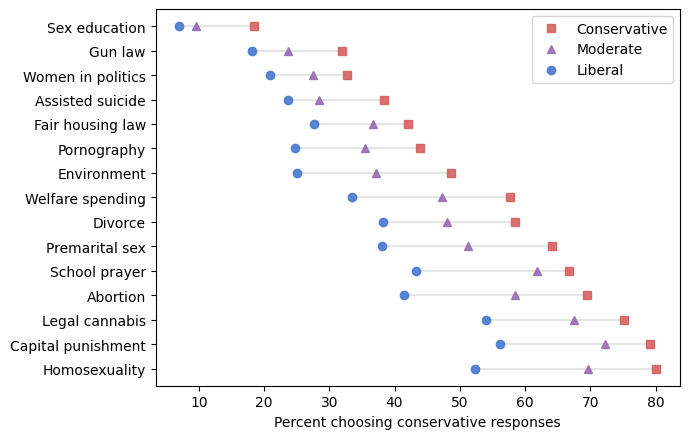
_images/eb401606ebc716c15615adcd28cb3913bc07c594a71824fd7cbd09a8c2ada195.png

Not surprisingly, conservatives are more likely than liberals to choose conservative responses, and moderates are somewhere in the middle. The differences between the groups range from 11 to 27 percentage points.

These results include respondents over the interval from 1973 to 2021, so they are not a snapshot of recent conditions. Rather, they show the issues that have distinguished conservatives from liberals over the last 50 years.

Item Response Theory#

Now that we’ve chosen questions that distinguish liberals and conservatives, the next step is to estimate the conservatism of each respondent. If all respondents answered all of the questions, this would be relatively easy, but they didn’t.

Some were surveyed before a particular question was added to the survey or after it was removed. Also, in some years respondents were randomly assigned a “ballot” with subset of the questions. Finally, a small percentage of respondents refuse to answer some questions, or say “I don’t know”.

The following figure shows the distribution of the number of questions answered.

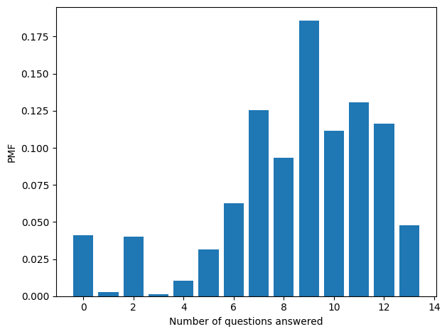
_images/322773b6bc4d3ab10332077938528a868f0d63cb8d43945bc7f96dbc513dd13c.png

Most respondents answered at least 5 questions, which is enough to get a sense of how conservative they are. But there’s another problem: some questions are “easier” than others. For some questions a majority choose a conservative response; for others it’s a small minority. If two people answer a different subject of the questions, we can’t compare them directly.

However, this is exactly the problem item response theory (IRT) is intended to solve! The fundamental assumptions of IRT are:

Each question has some level of difficulty, \(d_j\).
Each respondent has some level of efficacy, \(e_i\).
The probability that a respondent gets a question right is a function of \(d_j\) and \(e_i\).

In this context, a question is “difficult” if few people choose a conservative response and “easy” if many do. And if a respondent has high “efficacy”, that means they have a high tendency to choose conservative responses.

In one simple version of IRT, if a person with efficacy \(e_i\) answers a question with difficulty \(d_j\), the probability they get it right is

\[ \operatorname{expit}~(e_i - d_j)\]

Efficacy and difficulty are latent attributes; that is, we don’t observe them directly. Rather, we infer them from data. In some models, we use a large dataset to estimate \(e\) for each respondent and \(d\) for each question simultaneously. For this problem, that would be impractical, so I’ll use a shortcut: I’ll use the data to assign a difficulty to each question. Then I can estimate the efficacy of each respondent independently, which is simple and fast.

For each question, we know the proportion of respondents who chose a conservative response, which I’ll call \(p_j\).

To assign a difficulty to each question, I’ll use this heuristic: the difficulty of a question, \(d_j\), is the value so that if the question is answered by someone with \(e=0\), the probability they get it “right” is \(p_j\). This heuristic leads to the assignment:

\[ d_j = -\operatorname{logit}~(p_j) \]

The following figure shows these values for the fifteen questions.

from scipy.special import logit

ds = -logit(questions.mean().values)
ds

array([-0.82635786, -0.84985535, -0.74091316, -0.33876177, -0.36033642,
       -0.13601089,  0.03624691,  0.13082767,  0.49101244,  0.55948995,
        0.50827941,  0.77718599,  0.93359959,  1.0984166 ,  1.96117197])

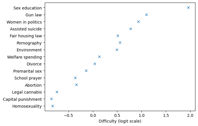
_images/c92401ec10fb3793347cb1e32797207b47b3a158a16a03bb569701ade24dea62.png

Where \(p_j\) is low, \(d_j\) is high. The range of these values, by itself, doesn’t mean very much; what matters is how the values of \(e\) and \(d\) relate to each other.

Given the assigned difficulties, we can identify a useful range of values for efficacy. The following figure shows the range I used, from -6 to 6.

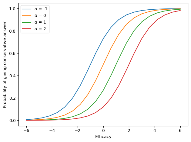
_images/966caadf1106810878f21217def8f56d10a3ba6e848e47cb52554d00f9a61713.png

Someone with efficacy -6 is very liberal; their probability of choosing a conservative response is nearly 0, even for the easiest question (\(d = -1\)). Someone with efficacy 6 is very conservative; their probability of choosing a conservative responses is nearly 1, even for the most difficulty question (\(d = 2\)).

Given the difficulties of the questions, we can compute the expected number of conservative responses at each level of efficacy.

E, D = np.meshgrid(es, ds)
P = expit(E - D)
ns = P.sum(axis=0)
plt.plot(es, ns)

decorate(xlabel="Efficacy", ylabel="Number of conservative answers")

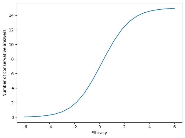
_images/7dbbe889bcdd2e27caa26b14beef8f9fb4c2debbb16c3768d1c72f92ee3d112c.png

Someone with efficacy 0 is expected to give about 7 conservative responses out of 15 questions.

Estimating Conservatism#

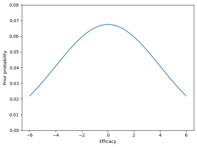
Now let’s see how we can estimate \(e_i\) for a respondent based on their answers. I’ll start with a (very) weakly informative prior that suggests people are more likely to be in the middle and less likely to be at the extremes.

from scipy.stats import norm
from empiricaldist import Pmf

ps = norm.pdf(es, 0, 4)
prior = Pmf(ps, es)
prior.normalize()
prior.plot()
decorate(xlabel="Efficacy", ylabel="Prior probability", ylim=[0, 0.08])

_images/b880307b1779944930adc4fee05a09759a43de8965ec16fdce2d61f6501de147.png

To demonstrate the estimation process, I’ll use the responses from an arbitrarily-chosen respondent.

row = questions.iloc[5000]
row

homosex     NaN
cappun      1.0
grass       0.0
abany       NaN
prayer      0.0
premarsx    1.0
divlaw      1.0
natfare     0.0
natenvir    1.0
pornlaw     0.0
racopen     1.0
letdie1     NaN
fepol       0.0
gunlaw      1.0
sexeduc     0.0
Name: 5034, dtype: float64

To compute the likelihood of the data, I’ll make an array, P, with one row per question and one column for each hypothetical value of \(e\). Each element of P is the probability that someone with a given efficacy gets a given question “right”.

E, D = np.meshgrid(es, ds)
P = expit(E - D)
Q = 1 - P
Q.shape

(15, 21)

Q is the complement of P; each element is the probability that someone with a given efficacy gets a given question “wrong”.

Now, for a given row of responses we can compute the likelihood of the data.

# compute the likelihoods of the conservative responses
index1 = np.nonzero(row.values == True)
like1 = P[index1]

# compute the likelihoods of the non-conservative responses
index2 = np.nonzero(row.values == False)
like2 = Q[index2]

# multiply them all together
like = np.vstack([like1, like2]).prod(axis=0)

like contains the likelihood of the data for each value of \(e\).

To do the Bayesian update, we multiply the prior by the likelihood and normalize. I’m using ns as the index of the posterior PMF, so the results are expressed in terms of the number of conservative responses, which is easier to interpret than efficacy.

posterior = Pmf(prior.values * like, ns)
posterior.normalize()
posterior.mean(), posterior.std()

(7.746546988198355, 1.9404648754849896)

Here’s what the posterior distribution looks like.

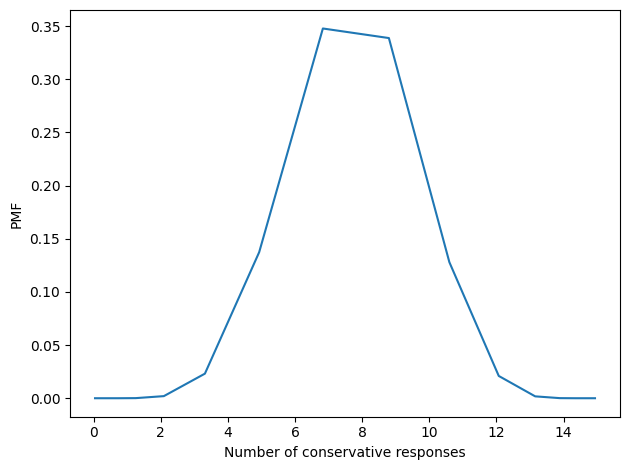
_images/a796f002fe9ad45aec27cee9eea34a95e397129522a979a14f8b24e512241fe3.png

The posterior mean is about 7.8 questions, but the spread of the distribution is wide, indicating that we are still uncertain about how conservative this respondent is.

Here’s the same code in a function.

So we can apply it to the whole dataset row-wise.

%time res = questions.apply(estimate_conservatism, axis=1, result_type='expand')
mean, std = np.transpose(res.values)

CPU times: user 27.1 s, sys: 293 ms, total: 27.4 s
Wall time: 27.1 s

Doing the calculation one row at a time takes longer than I’d like. So before we look at the results, let’s speed it up.

Array Operations For Speed#

To eliminate the apply function, we can compute the results for all respondents with a single 3-D array: one row for each respondent, one column for each question, one page for each hypothetical value of \(e\).

n, m = questions.shape
size = n, m, len(es)
res = np.empty(size)
res.shape

(71618, 15, 21)

Now we can fill the array with the likelihoods of conservative and non-conservative responses; where there’s a NaN, we fill in 1 (the identity of multiplication).

a = questions.fillna(2).astype(int).values
ii, jj = np.nonzero(a == 0)
res[ii, jj, :] = Q[jj]
ii, jj = np.nonzero(a == 1)
res[ii, jj, :] = P[jj]
ii, jj = np.nonzero(a == 2)
res[ii, jj, :] = 1

Multiplying along the rows gives the likelihood of each row of responses, which we multiply by the prior probabilities:

product = res.prod(axis=1) * prior.values
product.shape

(71618, 21)

Finally, we normalize the rows to get a posterior distribution for each respondent.

posterior = product / product.sum(axis=1)[:, None]
posterior.shape

(71618, 21)

The estimated conservatism for each respondent is the mean of the posterior distribution.

con = (posterior * ns).sum(axis=1)
con.shape

(71618,)

We’ll also compute the standard deviation of the posterior distribution, which quantifies the precision of the estimates.

deviations = ns - con[:, None]
var_con = (posterior * deviations ** 2).sum(axis=1)
std_con = np.sqrt(var_con)
std_con.shape

(71618,)

We can confirm that the results from the array operation is the same as the row-wise calculation.

assert np.allclose(con, mean)
assert np.allclose(std_con, std)

Here’s what the distribution of estimates looks like among the respondents.

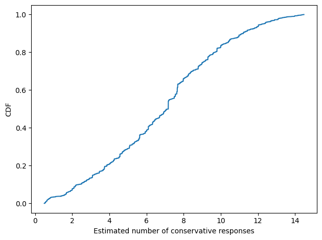
_images/2bd6fd49922541955e9a246662911dfbcb40d049653d914543932929581c9b86.png

con.mean()

6.855868381255202

The distribution is roughly Gaussian, with a mean near 7 questions. Here’s the distribution of standard deviations.

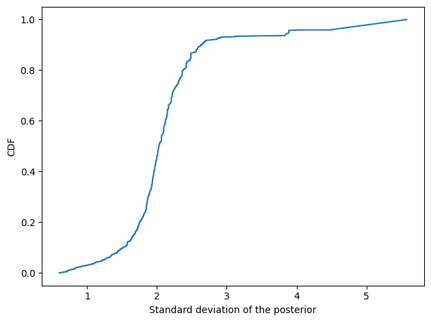
_images/16ad33c177f10820e4528eb734db69590f6ab5fc34f1cedbb0ceda31beb11c2a.png

For most respondents (about 63,000 out of 68,000) we have enough data to estimate the number of conservative responses with standard deviation less than 3.

In one version of this analysis, I excluded people based on this estimate of precision, but I think that introduces a bias because the estimates are more “precise” at the extremes.

In the current version, I exclude people based on the number of questions they answered.

answered = questions.notna().sum(axis=1)
np.percentile(answered, [10, 90])

array([ 5., 12.])

(answered >= 5).mean()

0.904283839258287

gss["conservatism"] = pd.Series(con, gss.index)
gss.loc[answered < 5, "conservatism"] = np.nan
gss["conservatism"].describe()

count    64763.000000
mean         6.833093
std          3.217315
min          0.494033
25%          4.524838
50%          6.838483
75%          9.302133
max         14.475336
Name: conservatism, dtype: float64

Conservatism Over Time#

The following figure shows the average of these estimates for each years of the survey.

series = gss.groupby("year")["conservatism"].mean()

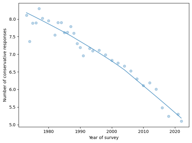
_images/e8c418d06a3a909b19a62ee711466aa473f7660336d1e0677469d0090f57d039.png

The prevalence of conservative responses has decreased over the last 50 years. In 1973, the average respondent chose a conservative response to 8.1 out of 15 questions; in 2021, it had fallen to 5.3.

There is no evidence that this trend has slowed or reversed recently. In 2012 and 2014, it might have been above the long-term trend; in 2016 and 2018, it was below it. And the most recent data, from 2021, is exactly on pace.

Are We Polarized?#

In current commentary, it is often taken for granted that politics in the U.S. have become more polarized. If we take that to mean that conservatives are becoming more conservative, and liberals more liberal, that turns out not to be true.

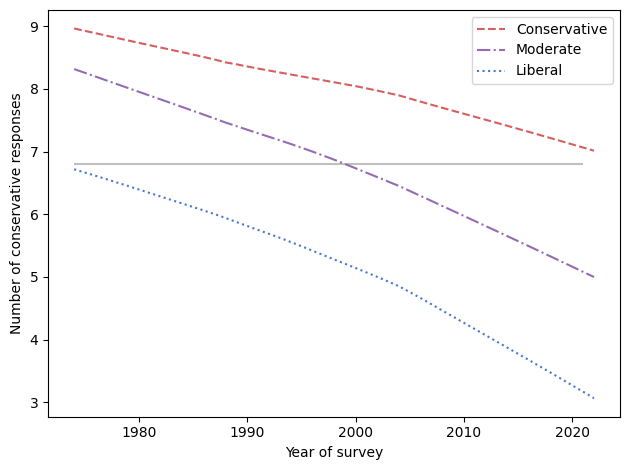
The following figure shows conservatism over time, grouped by political label.

table = gss.pivot_table(index="year", columns="polviews3", values="conservatism")

_images/08259367555b249a94f3a5599da8bd071fb029b8da3f8ec248cb71ab2c68e311.png

for column, series in table.items():
    smooth = make_lowess(series)
    diff = smooth.iloc[-1] - smooth.iloc[1]
    print(column, diff)

Conservative -1.9108828518012313
Liberal -3.5982851948518184
Moderate -3.2553493539659044

All three groups have become more liberal; however, the slopes of the lines are somewhat different. Over this interval, conservatives have become more liberal by about 1.9 expected responses, moderates by 3.1, and liberals by 3.4. That’s a kind of polarization in the sense that the groups moved farther apart, but not in the sense that they are moving in opposite directions.

In the previous figure, the horizontal line is at 6.8 responses, which was the expected level of conservatism in 1974 among people who called themselves liberal.

So, suppose you take a time machine back to 1974, find an average liberal, and bring them to the turn of the millennium. Based on their responses to the fifteen questions, they would be indistinguishable from the average moderate in 2000.

And if you bring them to 2021, their quaint 1970s liberalism would be almost as conservative as the average conservative.

Appendix: The Fifteen Questions#

This appendix provides the wording of the fifteen questions from the General Social Survey that most distinguish liberals and conservatives, identified by topic and the GSS variable name.

Homosexuality (homosex): What about sexual relations between two adults of the same sex–do you think it is always wrong, almost always wrong, wrong only sometimes, or not wrong at all?
Capital punishment (cappun): Do you favor or oppose the death penalty for persons convicted of murder?
Legal cannabis (grass): Do you think the use of marijuana should be made legal or not?
Abortion (abany): Please tell me whether or not you think it should be possible for a pregnant woman to obtain a legal abortion if the woman wants it for any reason?
Prayer in public schools (prayer): The United States Supreme Court has ruled that no state or local government may require the reading of the Lord’s Prayer or Bible verses in public schools. What are your views on this–do you approve or disapprove of the court ruling?
Premarital sex (premarsx): There’s been a lot of discussion about the way morals and attitudes about sex are changing in this country. If a man and woman have sex relations before marriage, do you think it is always wrong, almost always wrong, wrong only sometimes, or not wrong at all?
Divorce (divlaw): Should divorce in this country be easier or more difficult to obtain than it is now?
Spending on welfare (natfare) and the environment (natenvir): We are faced with many problems in this country, none of which can be solved easily or inexpensively. I’m going to name some of these problems, and for each one I’d like you to tell me whether you think we’re spending too much money on it, too little money, or about the right amount.
1. Welfare
2. Improving and protecting the environment
Pornography (pornlaw): Which of these statements comes closest to your feelings about pornography laws?
1. There should be laws against the distribution of pornography whatever the age.
2. There should be laws against the distribution of pornography to persons under 18.
3. There should be no laws forbidding the distribution of pornography.
Open housing law (racopen): Suppose there is a community-wide vote on the general housing issue. There are two possible laws to vote on; which law would you vote for?
1. One law says that a homeowner can decide for himself whom to sell his house to, even if he prefers not to sell to [people of a particular race].
2. The second law says that a homeowner cannot refuse to sell to someone because of their race or color.
Assisted suicide (letdie1): When a person has a disease that cannot be cured, do you think Doctors should be allowed by law to end the patient’s life by some painless means if the patient and his family request it?
Women in politics (fepol): Tell me if you agree or disagree with this statement: Most men are better suited emotionally for politics than are most women.
Gun control (gunlaw): Would you favor or oppose a law which would require a person to obtain a police permit before he or she could buy a gun?
Sex education (sexeduc): Would you be for or against sex education in the public schools?