You can order print and ebook versions of Think Bayes 2e from Bookshop.org and Amazon.
The Raven Paradox#
Suppose you are not sure whether all ravens are black. If you see a white raven, that clearly refutes the hypothesis. And if you see a black raven, that supports the hypothesis in the sense that it increases our confidence, maybe slightly. But what if you see a red apple – does that make the hypothesis any more or less likely?
This question is the core of the Raven Paradox, a problem in the philosophy of science posed by Carl Gustav Hempel in the 1940s. It highlights a counterintuitive aspect of how we evaluate evidence and confirm hypotheses.
No resolution of the paradox is universally accepted, but the most widely accepted is what I will call the standard Bayesian response. In this article, I’ll present this response, explain why I think it is incomplete, and propose an extension that might resolve the paradox.
Click here to run this notebook on Colab.
The Problem#
The paradox starts with the hypothesis
A: All ravens are black
And the contrapositive hypothesis
B: All non-black things are non-ravens
Logically, these hypotheses are identical – if A is true, B must be true, and vice versa. So if we have a certain level of confidence in A, we should have exactly the same confidence in B. And if we observe evidence in favor of A, we should also accept it as evidence in favor of B, to the same degree.
Also, if we accept that a black raven is evidence in favor of A, we should also accept that a non-black non-raven is evidence in favor of B.
Finally, if a non-black non-raven is evidence in favor of B, we should also accept that it is evidence in favor of A.
Therefore, a red apple (which is a non-black non-raven) is evidence that all ravens are black.
If you accept this conclusion, it seems like every time you see a red apple (or a blue car, or a green leaf, etc.) you should think, “Now I am slightly more confident that all ravens are black (and all flamingos are pink, etc.)”.
But that seems absurd, so we have two options:
Discover an error in the argument, or
Accept the conclusion.
As you might expect, many versions of (1) and (2) have been proposed.
The standard Bayesian response is to accept the conclusion but, quoth Wikipedia “argue that the amount of confirmation provided is very small, due to the large discrepancy between the number of ravens and the number of non-black objects. According to this resolution, the conclusion appears paradoxical because we intuitively estimate the amount of evidence provided by the observation of a green apple to be zero, when it is in fact non-zero but extremely small.”
It is true that when the number of non-ravens is large, the amount of evidence we get from each non-black non-raven is so small it is negligible. But I don’t think that’s why the conclusion is so acutely counterintuitive.
To clarify my objection, let me present a smaller example I’ll call the Roulette paradox.
An American roulette wheel has 36 pockets with the numbers 1 to 36, and two pockets labeled 0 and 00.
The non-zero pockets are red or black, and the zero pockets are green.
Suppose we work in quality control at the roulette factory and our job is to check that all zero pockets are green. If we observe a green zero, that’s evidence that all zeros are green. But what if we observe a red 19?
In this example, the standard Bayesian response fails:
First, the number of non-zeros is not particularly large, so the weight of the evidence is not negligible.
Also, the Bayesian response doesn’t address what I think is actually the key: The non-green non-zero may or may not be evidence, depending on how it was sampled.
As I will demonstrate,
If we choose a pocket at random and it turns out to be a non-green non-zero, that is not evidence that all zeros are green.
But if we choose a non-green pocket and it turns out to be non-zero, that is evidence that all zeros are green.
In both cases we observe a non-green non-zero, but “observe” is ambiguous. Whether the observation is evidence or not depends on the sampling process that generated the observation. And I think confusion between these two scenarios is the foundation of the paradox.
The Setup#
Let’s get into the details. Switching from roulette back to ravens, we will consider four scenarios:
You choose a random thing and it turns out to be a black raven.
You choose a random thing and it turns out to be a non-black non-raven.
You choose a random raven and it turns out to be black.
You choose a random non-black thing and it turns out to be a non-raven.
The key to the Raven Paradox is the difference between scenarios 2 and 4.
Scenario 2 is what most people imagine when they picture “observing a red apple”. And in this scenario, the red apple is irrelevant, exactly as intuition insists.
In Scenario 4, a red apple is evidence in favor of A, because we’re systematically checking non-black things to ensure they’re not ravens – so finding they aren’t is confirmation. But this sampling process is a more contrived interpretation of “observing a red apple”.
The reason for the paradox is that we imagine Scenario 2 and we are given the conclusion from Scenario 4.
It might not be obvious why the red apple is evidence in Scenario 4, but not Scenario 2. I think it will be clearer if we do the math.
The Math#
We’ll start with a small world where there are only N = 9 ravens and M = 19 non-ravens.
Then we’ll see what happens as we vary N and M.
N = 9
M = 19
I’ll use i to represent the unknown number of black ravens, which could be any value from 0 to N, and j to represent the unknown number of black non-ravens, from 0 to M.
We’ll use a joint distribution to represent beliefs about i and j; then we’ll use Bayes’s Theorem to update these beliefs when we see new data.
Let’s start with a uniform prior over all possible combinations of (i, j).
from empiricaldist import Pmf

def make_prior(N, M):
    prior_i = Pmf(1, np.arange(N + 1))
    prior_j = Pmf(1, np.arange(M + 1))
    prior = make_joint(prior_i, prior_j)
    normalize(prior)
    return prior
prior = make_prior(N, M)
The result is a Pandas DataFrame with the values of i across the columns and the values of j down the rows.
If i = N, that means all ravens are black, so we can compute the prior probability of A like this.
prior_A = prior[N].sum()
prior_A
0.10000000000000002
For this prior, the probability of A is 10%.
We’ll see later that the prior affects the strength of the evidence, but it doesn’t affect whether an observation is in favor of A or not.
Scenario 1#
Now let’s consider the first scenario: we choose a thing at random from the universe of things, and we find that it is a black raven.
The likelihood for this observation is: i / (N + M), because i is the number of black ravens and N + M is the total number of things.
The following function computes the posterior distribution of i and j in this scenario.
def update_scenario1(prior, N, M):
    # Create meshgrids for i and j
    I, J = make_mesh(prior)

    # Compute likelihood for Scenario 1
    likelihood = I / (N + M)

    # Perform Bayesian update
    posterior = prior * likelihood
    normalize(posterior)

    return posterior
Here’s the update.
posterior = update_scenario1(prior, N, M)
And here’s the posterior probability of A.
posterior_A = posterior[N].sum()
posterior_A
0.20000000000000004
The posterior probability is higher, so the black raven is evidence in favor of A.
To quantify the strength of the evidence, we’ll use the log odds ratio.
from scipy.special import logit

def log_odds_ratio(posterior_A, prior_A):
    return logit(posterior_A) - logit(prior_A)
lor = log_odds_ratio(posterior_A, prior_A)
lor
0.8109302162163288
Later we’ll see how the strength of the evidence depends on the prior distribution of i and j.
Before we go on, let’s also look at the marginal distribution of i (number of black ravens) before and after.
marginal_i_prior = marginal(prior, axis=0)
marginal_i_posterior = marginal(posterior, axis=0)
marginal_i_prior.plot(label='Prior', alpha=0.7)
marginal_i_posterior.plot(label='Posterior (Scenario 1)', alpha=0.7)
decorate(xlabel='Number of black ravens (i)',
         ylabel='Probability')
plt.savefig('raven_scenario1_marginal.png', dpi=150)
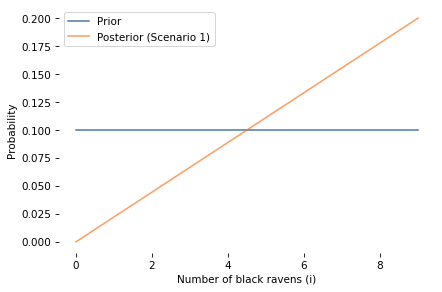
As expected, observing a black raven increases our confidence that all ravens are black.
The posterior distribution shifts toward higher values of i, and the probability that i = N increases.
In Scenario 1, the likelihood depends only on i, not on j, so the update doesn’t change our beliefs about j (the number of black non-ravens).
We can verify this by comparing the prior and posterior distributions of j:
marginal_j_prior = marginal(prior, axis=1)
marginal_j_posterior = marginal(posterior, axis=1)

np.allclose(marginal_j_prior, marginal_j_posterior)
True
Finally, let’s visualize posterior joint distribution of i and j.
def plot_joint(joint):
    # Transpose so i (number of black ravens) is on y-axis
    plt.imshow(joint.T, cmap='Blues')
    plt.gca().invert_yaxis()
    decorate(xlabel='Number of black non-ravens (j)',
             ylabel='Number of black ravens (i)')
plot_joint(posterior)
plt.title('Posterior: Scenario 1')
plt.savefig('raven_scenario1.png', dpi=150)
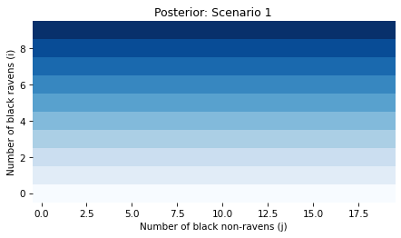
Because we started with a uniform distribution and the data has no bearing on j, the joint posterior probabilities don’t depend on j.
In summary, Scenario 1 is consistent with intuition: a black raven is evidence in favor of A.
Scenario 2#
In this scenario, we choose a thing at random from the universe of N + M things, and it turns out to be a red apple – which we will treat generally as a non-black non-raven.
The likelihood of this observation is: (M - j) / (N + M), because M - j is the number of non-black non-ravens and N + M is the total number of things.
The following function computes the posterior distribution of i and j in this scenario.
def update_scenario2(prior, N, M):
    # Create meshgrids for i and j
    I, J = make_mesh(prior)

    # Compute likelihood for Scenario 2
    likelihood = (M - J) / (N + M)

    # Perform Bayesian update
    posterior = prior * likelihood
    normalize(posterior)

    return posterior
Here’s the update.
posterior = update_scenario2(prior, N, M)
And here’s the posterior probability of A.
posterior_A = posterior[N].sum()
posterior_A
0.1
In this scenario, the posterior probability of A is the same as the prior.
In fact, the entire distribution of i is unchanged.
marginal_i_prior = marginal(prior, axis=0)
marginal_i_posterior = marginal(posterior, axis=0)

np.allclose(marginal_i_prior, marginal_i_posterior)
True
So the red apple is not evidence in favor of A or against it.
This is consistent with the intuition that the red apple (or any non-black non-raven) is irrelevant.
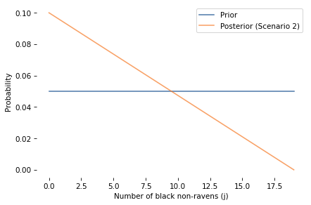
However, the red apple is evidence about j, as we can confirm by comparing the marginal distribution of j before and after.
marginal_j_prior = marginal(prior, axis=1)
marginal_j_posterior = marginal(posterior, axis=1)
marginal_j_prior.plot(label='Prior', alpha=0.7)
marginal_j_posterior.plot(label='Posterior (Scenario 2)', alpha=0.7)
decorate(xlabel='Number of black non-ravens (j)',
         ylabel='Probability')
plt.savefig('raven_scenario2_marginal.png', dpi=150)
And here’s the posterior joint distribution of i and j.
plot_joint(posterior)
plt.title('Posterior: Scenario 2')
plt.savefig('raven_scenario2.png', dpi=150)
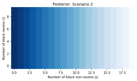
Because the red apple has no bearing on i, the posterior probabilities in this scenario don’t depend on i.
In summary, Scenario 2 matches our intuition: a red apple (chosen at random) is not evidence about whether all ravens are black.
Scenario 3#
In this scenario, we choose a raven first and then observe that it is black.
The likelihood for this observation is: i / N, because i is the number of black ravens and N is the total number of ravens.
The following function computes the posterior distribution of i and j in this scenario.
def update_scenario3(prior, N, M):
    # Create meshgrids for i and j
    I, J = make_mesh(prior)

    # Compute likelihood for Scenario 3
    likelihood = I / N

    # Perform Bayesian update
    posterior = prior * likelihood
    normalize(posterior)

    return posterior
Here’s the update.
posterior = update_scenario3(prior, N, M)
And here’s the posterior probability of A.
posterior_A = posterior[N].sum()
posterior_A
0.20000000000000004
This posterior is the same as in Scenario 1, so we conclude that the black raven is evidence in favor of A, with the same strength regardless of whether we are in:
Scenario 1: Select a random thing and it turns out to be a black raven or
Scenario 3: Select a random raven and it turns out to be black.
In fact, the entire posterior distribution is the same in both scenarios. That’s because the likelihoods in Scenarios 1 and 3 differ only by a constant factor, which is removed when the posterior distributions are normalized.
In summary, Scenario 3 is consistent with intuition: if we choose a raven and find that it is black, that is evidence in favor of A.
Scenario 4#
In the last scenario, we first choose a non-black thing (from all non-black things in the universe), and then observe that it is a non-raven.
The likelihood of this observation is: (M - j) / (N - i + M - j) because M - j is the number of non-black non-ravens and N - i + M - j is the total number of non-black things.
This likelihood depends on both i and j, unlike Scenario 2.
This is the key difference that makes Scenario 4 informative about whether all ravens are black.
The following function computes the posterior distribution of i and j in this scenario.
def update_scenario4(prior, N, M):
    # Create meshgrids for i and j
    I, J = make_mesh(prior)

    # Compute likelihood for Scenario 4
    with np.errstate(invalid='ignore'):
        likelihood = (M - J) / (N - I + M - J)

    # Perform Bayesian update
    posterior = prior * np.nan_to_num(likelihood)
    normalize(posterior)

    return posterior
Here’s the update.
posterior = update_scenario4(prior, N, M)
And here’s the posterior probability of A.
posterior_A = posterior[N].sum()
posterior_A
0.14940297326954258
The posterior is greater than the prior, so the non-black non-raven is evidence in favor of A.
Again, we can quantify the strength of the evidence by computing the log odds ratio.
lor = log_odds_ratio(posterior_A, prior_A)
lor
0.45793326392280087
The LOR is smaller than in Scenarios 1 and 3, because there are more non-ravens than ravens.
As we’ll see, the strength of the evidence gets smaller as M gets bigger.
Here is the marginal distribution of i (number of black ravens) before and after:
marginal_i_prior = marginal(prior, axis=0)
marginal_i_posterior = marginal(posterior, axis=0)
marginal_i_prior.plot(label='Prior', alpha=0.7)
marginal_i_posterior.plot(label='Posterior (Scenario 4)', alpha=0.7)
decorate(xlabel='Number of black ravens (i)',
         ylabel='Probability')
plt.savefig('raven_scenario4_marginal_i.png', dpi=150)

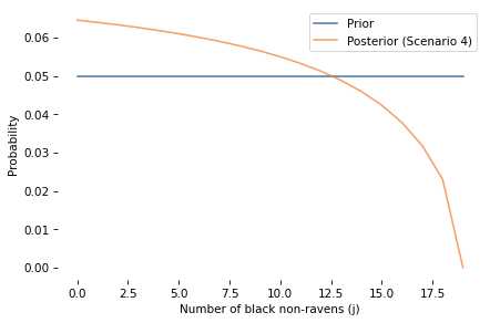
And here’s the marginal distribution of j (number of black non-ravens) before and after.
marginal_j_prior = marginal(prior, axis=1)
marginal_j_posterior = marginal(posterior, axis=1)
marginal_j_prior.plot(label='Prior', alpha=0.7)
marginal_j_posterior.plot(label='Posterior (Scenario 4)', alpha=0.7)
decorate(xlabel='Number of black non-ravens (j)',
         ylabel='Probability')
plt.savefig('raven_scenario4_marginal_j.png', dpi=150)
Finally, here’s the posterior joint distribution of i and j.
plot_joint(posterior)
plt.title('Posterior: Scenario 4')
plt.savefig('raven_scenario4.png', dpi=150)
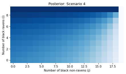
In Scenario 4, the likelihood depends on both i and j, so the update changes our beliefs about both parameters.
And in Scenario 4 a non-black non-raven (chosen from non-black things) is evidence in favor of A.
This might still be surprising, but let me suggest a way to think about it: in this scenario we are checking non-black things to make sure they are not ravens.
If we find a non-black raven, that contradicts A.
If we don’t, that supports A.
In all four scenarios, the results are consistent with intuition. So as long as you are clear about which scenario you are in, there is no paradox. The paradox is only apparent if you think you are in Scenario 2 and you imagine the result from Scenario 4.
In the context of the original problem:
If you walk out of your house and the first thing you see is a red apple (or a blue car, or a green leaf) that has no bearing on whether raven are black.
But if you deliberately select a non-black thing and check whether it’s a raven, and you find that it is not, that actually is evidence that all ravens are black – but consistent with the standard Bayesian response, it is so weak it is negligible.
Successive updates#
In these examples, we started with a uniform prior over all combinations of i and j.
Of course that’s not a realistic representation of what we believe about the world.
So let’s consider the effect of other priors.
In general, different priors lead to different posterior distributions, and in this case they lead to different conclusions about the strength of the evidence. But they lead to the same conclusion about the direction of the evidence.
To demonstrate, let’s see what happens if we observe a series of black ravens (in Scenario 1 or 3). For simplicity, assume that we sample with replacement.
The following function computes multiple updates, starting with the uniform prior and then using the posterior from each update as the prior for the next.
def multiple_updates(prior, update_func, N, M, iters=10):
    joint = prior.copy()
    res = []
    for i in range(iters):
        prior_A = joint[N].sum()
        joint = update_func(joint, N, M)
        posterior_A = joint[N].sum()
        res.append((prior_A, posterior_A))

    return make_table(res)

def make_table(res, columns=['Prior', 'Posterior']):
    res_df = pd.DataFrame(res, columns=columns)
    res_df['LOR'] = log_odds_ratio(res_df['Posterior'], res_df['Prior'])
    res_df.index.name = 'Iteration'
    return res_df
This table shows the results in Scenario 1 (which is the same as in Scenario 3).
For each iteration, the table shows the prior and posterior probability of A, and the log odds ratio.
multiple_updates(prior, update_scenario1, N, M).round(3)
| Prior | Posterior | LOR | |
|---|---|---|---|
| Iteration | |||
| 0 | 0.100 | 0.200 | 0.811 |
| 1 | 0.200 | 0.284 | 0.463 |
| 2 | 0.284 | 0.360 | 0.348 |
| 3 | 0.360 | 0.428 | 0.285 |
| 4 | 0.428 | 0.489 | 0.245 |
| 5 | 0.489 | 0.543 | 0.218 |
| 6 | 0.543 | 0.592 | 0.199 |
| 7 | 0.592 | 0.636 | 0.184 |
| 8 | 0.636 | 0.675 | 0.173 |
| 9 | 0.675 | 0.710 | 0.164 |
As we see more ravens, the posterior probability of A increases, but the LOR decreases – which means that each raven provides weaker evidence than the previous one.
In the long run the LOR converges to a value greater than 0 (about 0.11), which means that each raven provides at least some additional evidence, even when the prior is far from the uniform distribution we started with.
In the worst case, if the prior probability of A is 0 or 1, nothing we observe can change those beliefs, so nothing is evidence for or against A.
But there is no prior where a black raven provides evidence against A.
[Proof: The likelihood of the observation is maximized when all ravens are black (i = N). Therefore, for any prior that gives non-zero probability to both A and its complement, the LOR is positive: these observations can never be evidence against A.]
The following table shows the results in Scenario 4, where we select a non-black thing and check that it is not a raven.
multiple_updates(prior, update_scenario4, N, M).round(3)
| Prior | Posterior | LOR | |
|---|---|---|---|
| Iteration | |||
| 0 | 0.100 | 0.149 | 0.458 |
| 1 | 0.149 | 0.201 | 0.359 |
| 2 | 0.201 | 0.254 | 0.303 |
| 3 | 0.254 | 0.307 | 0.264 |
| 4 | 0.307 | 0.359 | 0.236 |
| 5 | 0.359 | 0.410 | 0.213 |
| 6 | 0.410 | 0.458 | 0.194 |
| 7 | 0.458 | 0.502 | 0.179 |
| 8 | 0.502 | 0.543 | 0.166 |
| 9 | 0.543 | 0.582 | 0.155 |
The pattern is similar.
Each non-black thing that turns out not to be a raven is weaker evidence than the previous one.
But it is always in favor of A – in this scenario, there is no prior where a non-black non-raven is evidence against A.
Varying M#
Finally, let’s see how the strength of the evidence varies as we increase M, the number of non-ravens.
The following function computes results in Scenario 4 for a range of values of M, holding constant the number of ravens, N = 9.
def update_with_varying_M(N, M_values):
    """Run Scenario 4 for different values of M."""
    res = []

    for M in M_values:
        prior = make_prior(N, M)
        prior_A = prior[N].sum()
        posterior = update_scenario4(prior, N, M)
        posterior_A = posterior[N].sum()
        res.append((M, prior_A, posterior_A))

    table = make_table(res, columns=['M', 'Prior', 'Posterior'])
    return table.set_index('M')
M_values = [20, 50, 100, 200, 500, 1000]
update_with_varying_M(N, M_values).round(3)
| Prior | Posterior | LOR | |
|---|---|---|---|
| M | |||
| 20 | 0.1 | 0.148 | 0.444 |
| 50 | 0.1 | 0.125 | 0.247 |
| 100 | 0.1 | 0.115 | 0.152 |
| 200 | 0.1 | 0.108 | 0.091 |
| 500 | 0.1 | 0.104 | 0.045 |
| 1000 | 0.1 | 0.102 | 0.026 |
As M increases (more non-ravens in the universe), the strength of the evidence decreases.
This is consistent with the standard Bayesian response, which notes that in a realistic scenario, the evidence is negligible.
Conclusion#
The standard Bayesian response to the Raven Paradox is correct in the sense that if a non-black non-raven is evidence that all ravens are black, it is so extremely weak. But that doesn’t explain why the roulette example – where the number of non-green non-zero pockets is relatively small – is still so contrary to intuition.
I think a better explanation for the paradox is the ambiguity of the word “observe”. If we are explicit about the sampling process that generates the observation, we find that a non-black non-raven may or may not be evidence that all ravens are black.
Scenario 2: If we choose a random thing and find that it is a non-black non-raven, that is not evidence.
Scenario 4: If we choose a non-black thing and find that it is a non-raven, that is evidence.
The first case is entirely consistent with intuition. The second case is less obvious, but if we consider smaller examples like a roulette wheel, and do the math, it can be reconciled with intuition.
Confusion between these scenarios causes the apparent paradox, and clarity about the scenarios resolves it.
Symmetry and Asymmetry#
It might still seem strange that a black raven is always evidence for A and B, but a non-black non-raven may or may not be, depending on the sampling process.
If A and B are logically identical, and a black raven supports A, it’s still not clear why a non-black non-raven doesn’t always support B.
After all, if we start with B, we conclude that a non-black non-raven is always evidence for B (and A), and a black raven may or may not be.
Where does this asymmetry come from?
We broke the symmetry when we formulated “All ravens are black” as “Out of all ravens, how many are black?” This formulation first divides the world into ravens and non-ravens, then asks how many in each group are black.
Conversely, if we start with “All non-black things are non-ravens”, we formulate it as “Out of all non-black things, how many are ravens?” In this formulation, we divide the world into black and non-black things, then ask how many in each group are ravens.
The asymmetry is apparent when we parameterize the models.
If we start with A, we define i to be the number of ravens that are black.
And we find that in Scenario 1, the likelihood of a black raven depends on i, and in Scenario 2, the likelihood of a non-black non-raven does not.
If we start with B, we define i to be the number of non-black things that are non-ravens.
Then in Scenario 1 we find that a non-black non-raven pertains to i, but a black raven does not.
So the symmetry is broken when we formulate the hypothesis in a way that is testable with data.
In propositional logic, A and B are equivalent in the sense that evidence for one must be evidence for the other.
In the Bayesian formulation, “How many ravens are black?” and “How many non-black things are non-ravens?” are not equivalent; evidence for one is not necessarily evidence for the other.
A critic might say that the Bayesian formulation is a non-resolution – that is, it doesn’t solve the original problem posed by Hempel; it only solves a related problem by making additional assumptions.
A Bayesian response is that the Raven Paradox is only problematic in the abstract world of propositional logic; as soon as we formulate the question in a way that connects it to the real world through observation, it disappears. So the Raven Paradox is similar to the principle of explosion – it demonstrates a brittleness in propositional logic that makes it unsuitable for reasoning about many real-world hypotheses.
Objections#
Objection: In real life, we might not know which scenario we’re in when we observe something.
Response: True, but that’s the point. The paradox arises because we fail to recognize that different observation processes have different evidential implications. In practice, we should think carefully about how we encountered evidence before drawing conclusions. If you accidentally see a red apple, you’re in Scenario 2. If you’re systematically checking non-black things, you’re in Scenario 4.
Objection: Scenario 4 never actually happens in real life. No one deliberately samples non-black things to check if they’re ravens.
Response: That’s true in the raven example, but that’s because the evidence is so weak. In cases where M is smaller, selecting non-black things might be practical, especially if they are easier to find or easier to check.
Objection: This resolution still requires that we accept the counterintuitive conclusion in Scenario 4.
Response: Yes, but once you understand the sampling process, it’s not so counterintuitive. If you’re systematically checking non-black things to make sure none are ravens, finding that they aren’t ravens should increase your confidence that all ravens are black. The confusion arises only when we imagine Scenario 2 but apply Scenario 4’s conclusion.
Objection: The uniform prior over (i, j) is unrealistic.
Response: The prior affects the strength of the evidence but not its direction. As shown in the “Successive Updates” section, regardless of the prior (except for the degenerate cases of 0 or 1), black ravens always provide positive evidence for A, and in Scenario 4, non-black non-ravens always provide positive evidence. The qualitative conclusion is prior-independent.
Objection: This just pushes the problem back. Now we need a theory of when observations count as Scenario 2 vs. Scenario 4.
Response: Evidence interpretation always depends on understanding how the evidence was generated. Making this dependence explicit resolves the paradox rather than creating a new problem.
Objection: You’re conflating “all ravens are black” with “the proportion of black ravens is 1” which are logically different.
Response: For the purposes of Bayesian inference, we model the universal generalization probabilistically by considering the proportion of black ravens. This is a standard approach that allows us to update beliefs continuously. If you prefer to treat “all ravens are black” as strictly true or false, you lose the ability to model degrees of confirmation.
Objection: The roulette example doesn’t help because 38 pockets is still small compared to the universe of things.
Response: The point of the roulette example is to show that even with manageable numbers, the distinction between Scenario 2 and Scenario 4 still matters. If negligibility alone explained the paradox, the roulette case shouldn’t feel paradoxical – but it does until we clarify the sampling process.
Objection: Doesn’t this make confirmation theory hopelessly dependent on psychological facts about what observers intended?
Response: No, it makes confirmation properly dependent on the causal structure of how observations were generated, not on psychological intentions. Whether you randomly selected a thing or deliberately selected a non-black thing is an objective fact about your sampling procedure, not a subjective mental state.
Objection: This analysis is based on Bayesianism. What about other interpretations of probability and other models of confirmation?
Response: The paradox can be resolved under Bayesianism. If it can’t be resolved in an alternative framework, that seems like a problem for the alternative and a point in favor of Bayesianism.
Objection: Bayesian analysis is based on priors, so it’s subjective.
Response: Yes, Bayesian analysis is subjective, but only partly because of priors. It is also subjective because is it based on a model of the data generating process, and model selection is subjective. So avoiding priors is pointless: it limits what you can do without actually eliminating subjectivity.
Objection: From a correspondent: “The standard Bayesian solution posits a fixed number of ravens, non-ravens, and black objects and concludes correctly that a randomly sampled non-black non-raven sighting does change (slightly) the probability that all ravens are black (since that slightly increases the probability that the remaining objects, including all the ravens, are black).”
Response: Yes, there are other models of Scenario 2 where a non-black non-raven is evidence for A. I think that supports my claim that the conclusion depends on our model of the data-generating process. I won’t argue that my model is right – only that it is one example of a model where the conclusion is consistent with intuition.
Objection: The finite-world model assumes we know the total number of ravens and non-ravens (N and M). That’s unrealistic.
Response: I agree that it’s unrealistic for the raven example. But I think it’s a useful modeling strategy to treat them as known quantities and then see what happens as they get bigger.
An alternative is to treat N and M as unknown, assign priors, and update them along with i and j.
I haven’t done that analysis, but I think in that case a non-black non-raven might or might not be evidence for A, depending on the priors.
Again, this supports my claim that the conclusion depends on our model of the data-generating process, including the priors.
Objection: This analysis ignores background knowledge; for example, we already know apples are not ravens, so the likelihood of non-black non-raven observations is fixed by prior knowledge, not by the sampling model.
Response: Background knowledge can be incorporated into the joint prior over (i, j). Doing so changes the strength – but not the direction – of confirmation. Scenario 2 still yields no information about A, and Scenario 4 still yields a positive (albeit tiny) increment.
Objection: The analysis treats color and “raven-ness” as probabilistically independent dimensions, but real biological traits aren’t independent.
Response: In the uniform prior, i and j are independent, but in Scenario 4, they are no longer independent after the first update. If we have background knowledge about dependence between i and j, we can incorporate it in the prior. But again, different priors change the strength – but not the direction – of confirmation.
Objection: Isn’t the conclusion trivial? Of course sampling procedures matter. Why present this as a paradox?
Response: Sampling procedures matter, but the Raven paradox is specifically about the intuitive asymmetry between observing a black raven and observing a non-black non-raven. People treat these observations as categorically different, even when sampling processes are held constant. The “trivial” insight that sampling matters resolves the paradox precisely because the paradox arises when we implicitly substitute one sampling model for another without noticing it. Clarifying sampling assumptions dissolves the problem that seemed paradoxical.
Objection: Why not simply reject Hempel’s equivalence condition (that confirming a proposition also confirms its contrapositive)?
Response: Rejecting logical equivalence is a radical move: it breaks classical confirmation theory and undermines deductive coherence. The goal is not to change logic but to recognize that confirmation is not a purely logical relation; it is a probabilistic one. Under Bayesianism, logically equivalent hypotheses still receive the same degree of support when conditioned on the same observation under the same sampling model. The paradox dissolves once we see that “the same observation” refers to different sampling models in Scenarios 2 and 4.
Objection: Scenario 4 seems contrived – the observer already knows the object is non-black before checking whether it is a raven.
Response: Yes, it is contrived, which is why it is probably not the sampling process people imagine when they are told that we “observe” a non-black non-raven. And that’s the problem – in the more natural scenario, a red apple is not evidence, just as we expect. It is only evidence in the more contrived scenario.
Objection: Your model treats hypotheses as if they were about static populations. But universal generalizations are about laws, not frequencies.
Response: True, but Bayesian confirmation treats laws probabilistically by modeling them as statements about parameters. This is a standard and widely accepted practice. A law like “all ravens are black” is modeled as the claim that the proportion of black ravens is 1. This enables the use of likelihood and Bayes’s theorem to track how evidence shifts our degree of belief in the law. Rejecting this modeling strategy would simply make Bayesian confirmation impossible, not resolve the paradox.
Objection: You assume that all observations are equally reliable. What about observational error?
Response: Measurement error can be incorporated by modifying the likelihood functions. If observers sometimes misclassify color or species, the likelihoods in Scenarios 2 and 4 change. If the misclassification rate is high enough, it can reverse the sense of the evidence, so a raven classified as black might be evidence against A – but similarly a non-black thing classified as raven might be evidence in favor is A. Misclassification complicates the analysis but doesn’t contradict the conclusion that the paradox is resolved when we are explicit about the sampling process.
Objection: Why not use a continuous model for the proportion of black ravens instead of discrete counts?
Response: We could, and that’s how Royall formulated the model. In that case the argument about the direction of evidence is the same, and the update is similar, but we run into a problem when we use the posterior distribution to compute the probability of A. If the distribution of the proportion is continuous, the probability is 0 that the proportion is exactly 1. I don’t think that really changes the conclusion, but it makes the Bayesian formulation one more step removed from the original question, which might bother some people.
This notebook uses methods and materials from Think Bayes, second edition. If you like this sort of thing, you can read the whole book, and more examples, at allendowney.github.io/ThinkBayes2/.
Copyright 2025 Allen B. Downey
License: Attribution-NonCommercial-ShareAlike 4.0 International (CC BY-NC-SA 4.0)