Regression

Regression#

In the previous chapter we saw several examples of logistic regression, which is based on the assumption that the likelihood of an outcome, expressed in the form of log odds, is a linear function of some quantity (continuous or discrete).

In this chapter we’ll work on examples of simple linear regression, which models the relationship between two quantities. Specifically, we’ll look at changes over time in snowfall and the marathon world record.

The models we’ll use have three parameters, so you might want to review the tools we used for the three-parameter model in <<_MarkandRecapture>>.

More Snow?#

I am under the impression that we don’t get as much snow around here as we used to. By “around here” I mean Norfolk County, Massachusetts, where I was born, grew up, and currently live. And by “used to” I mean compared to when I was young, like in 1978 when we got 27 inches of snow and I didn’t have to go to school for a couple of weeks.

Fortunately, we can test my conjecture with data. Norfolk County happens to be the location of the Blue Hill Meteorological Observatory, which keeps the oldest continuous weather record in North America.

Data from this and many other weather stations is available from the National Oceanic and Atmospheric Administration (NOAA). I collected data from the Blue Hill Observatory from May 11, 1967 to May 11, 2020.

The following cell downloads the data as a CSV file.

We can use Pandas to read the data into DataFrame:

import pandas as pd

df = pd.read_csv('2239075.csv', parse_dates=[2])

Here’s what the last few rows look like.

Show code cell content Hide code cell content

df.tail(3)

	STATION	NAME	DATE	TMAX	TMIN	TOBS	WESD	WT01	WT03	WT04	WT05	WT06	WT08	WT09	WT11	WT16	WT18
20452	USC00190736	BLUE HILL COOP, MA US	2023-05-09	75	45.0	51.0	NaN	NaN	NaN	NaN	NaN	NaN	NaN	NaN	NaN	NaN	NaN
20453	USC00190736	BLUE HILL COOP, MA US	2023-05-10	60	42.0	51.0	NaN	NaN	NaN	NaN	NaN	NaN	NaN	NaN	NaN	NaN	NaN
20454	USC00190736	BLUE HILL COOP, MA US	2023-05-11	72	51.0	59.0	NaN	NaN	NaN	NaN	NaN	NaN	NaN	NaN	NaN	NaN	NaN

The columns we’ll use are:

DATE, which is the date of each observation,
SNOW, which is the total snowfall in inches.

I’ll add a column that contains just the year part of the dates.

df['YEAR'] = df['DATE'].dt.year

And use groupby to add up the total snowfall in each year.

snow = df.groupby('YEAR')['SNOW'].sum()

The first and last years are not complete, so I’ll drop them.

The following figure shows total snowfall during each of the complete years in my lifetime.

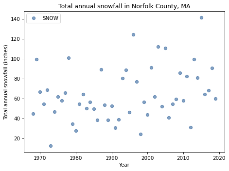
_images/a18b7ac97e8129afa56f1cc415d2c5d0e3cf9c07dd90c3fcc04552fe5632ef46.png

Looking at this plot, it’s hard to say whether snowfall is increasing, decreasing, or unchanged. In the last decade, we’ve had several years with more snow than 1978, including 2015, which was the snowiest winter in the Boston area in modern history, with a total of 141 inches.

This kind of question – looking at noisy data and wondering whether it is going up or down – is precisely the question we can answer with Bayesian regression.

Regression Model#

The foundation of regression (Bayesian or not) is the assumption that a time series like this is the sum of two parts:

A linear function of time, and
A series of random values drawn from a distribution that is not changing over time.

Mathematically, the regression model is

\[y = a x + b + \epsilon\]

where \(y\) is the series of measurements (snowfall in this example), \(x\) is the series of times (years) and \(\epsilon\) is the series of random values.

\(a\) and \(b\) are the slope and intercept of the line through the data. They are unknown parameters, so we will use the data to estimate them.

We don’t know the distribution of \(\epsilon\), so we’ll make the additional assumption that it is a normal distribution with mean 0 and unknown standard deviation, \(\sigma\).
To see whether this assumption is reasonable, I’ll plot the distribution of total snowfall and a normal model with the same mean and standard deviation.

Here’s a Pmf object that represents the distribution of snowfall.

from empiricaldist import Pmf

pmf_snowfall = Pmf.from_seq(snow)

And here are the mean and standard deviation of the data.

mean, std = pmf_snowfall.mean(), pmf_snowfall.std()
mean, std

(63.62363636363636, 25.851147072396568)

I’ll use the norm object from SciPy to compute the CDF of a normal distribution with the same mean and standard deviation.

from scipy.stats import norm

dist = norm(mean, std)
qs = pmf_snowfall.qs
ps = dist.cdf(qs)

Here’s what the distribution of the data looks like compared to the normal model.

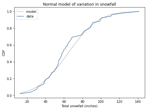
_images/d7b23964f610a03df17062f571da04796b630b921052f6c1b3cf18f64557c2f6.png

We’ve had more winters below the mean than expected, but overall this looks like a reasonable model.

Least Squares Regression#

Our regression model has three parameters: slope, intercept, and standard deviation of \(\epsilon\). Before we can estimate them, we have to choose priors. To help with that, I’ll use StatsModel to fit a line to the data by least squares regression.

First, I’ll use reset_index to convert snow, which is a Series, to a DataFrame.

data = snow.reset_index()
data.head(3)

	YEAR	SNOW
0	1968	44.7
1	1969	99.2
2	1970	66.8

The result is a DataFrame with two columns, YEAR and SNOW, in a format we can use with StatsModels.

As we did in the previous chapter, I’ll center the data by subtracting off the mean.

offset = round(data['YEAR'].mean())
data['x'] = data['YEAR'] - offset
offset

And I’ll add a column to data so the dependent variable has a standard name.

data['y'] = data['SNOW']

Now, we can use StatsModels to compute the least squares fit to the data and estimate slope and intercept.

import statsmodels.formula.api as smf

formula = 'y ~ x'
results = smf.ols(formula, data=data).fit()
results.params

Intercept    63.623636
x             0.376421
dtype: float64

The intercept, about 64 inches, is the expected snowfall when x=0, which is the beginning of 1994. The estimated slope indicates that total snowfall is increasing at a rate of about 0.5 inches per year.

results also provides resid, which is an array of residuals, that is, the differences between the data and the fitted line. The standard deviation of the residuals is an estimate of sigma.

results.resid.std()

25.382858670693558

We’ll use these estimates to choose prior distributions for the parameters.

Priors#

I’ll use uniform distributions for all three parameters.

import numpy as np
from utils import make_uniform

qs = np.linspace(-0.5, 1.5, 51)
prior_slope = make_uniform(qs, 'Slope')

qs = np.linspace(54, 75, 41)
prior_inter = make_uniform(qs, 'Intercept')

qs = np.linspace(20, 35, 31)
prior_sigma = make_uniform(qs, 'Sigma')

I made the prior distributions different lengths for two reasons. First, if we make a mistake and use the wrong distribution, it will be easier to catch the error if they are all different lengths.

Second, it provides more precision for the most important parameter, slope, and spends less computational effort on the least important, sigma.

In <<_ThreeParameterModel>> we made a joint distribution with three parameters. I’ll wrap that process in a function:

from utils import make_joint

def make_joint3(pmf1, pmf2, pmf3):
    """Make a joint distribution with three parameters."""
    joint2 = make_joint(pmf2, pmf1).stack()
    joint3 = make_joint(pmf3, joint2).stack()
    return Pmf(joint3)

And use it to make a Pmf that represents the joint distribution of the three parameters.

prior = make_joint3(prior_slope, prior_inter, prior_sigma)
prior.head(3)

			probs
Slope	Intercept	Sigma
-0.5	54.0	20.0	0.000015
		20.5	0.000015
		21.0	0.000015

The index of Pmf has three columns, containing values of slope, inter, and sigma, in that order.

With three parameters, the size of the joint distribution starts to get big. Specifically, it is the product of the lengths of the prior distributions. In this example, the prior distributions have 51, 41, and 31 values, so the length of the joint prior is 64,821.

Likelihood#

Now we’ll compute the likelihood of the data. To demonstrate the process, let’s assume temporarily that the parameters are known.

inter = 64
slope = 0.51
sigma = 25

I’ll extract the xs and ys from data as Series objects:

xs = data['x']
ys = data['y']

And compute the “residuals”, which are the differences between the actual values, ys, and the values we expect based on slope and inter.

expected = slope * xs + inter
resid = ys - expected

According to the model, the residuals should follow a normal distribution with mean 0 and standard deviation sigma. So we can compute the likelihood of each residual value using norm from SciPy.

densities = norm(0, sigma).pdf(resid)

The result is an array of probability densities, one for each element of the dataset; their product is the likelihood of the data.

likelihood = densities.prod()
likelihood

9.70222384229511e-112

As we saw in the previous chapter, the likelihood of any particular dataset tends to be small. If it’s too small, we might exceed the limits of floating-point arithmetic. When that happens, we can avoid the problem by computing likelihoods under a log transform. But in this example that’s not necessary.

The Update#

Now we’re ready to do the update. First, we need to compute the likelihood of the data for each possible set of parameters.

likelihood = prior.copy()

for slope, inter, sigma in prior.index:
    expected = slope * xs + inter
    resid = ys - expected
    densities = norm.pdf(resid, 0, sigma)
    likelihood[slope, inter, sigma] = densities.prod()

This computation takes longer than many of the previous examples. We are approaching the limit of what we can do with grid approximations.

Nevertheless, we can do the update in the usual way:

posterior = prior * likelihood
posterior.normalize()

The result is a Pmf with a three-level index containing values of slope, inter, and sigma. To get the marginal distributions from the joint posterior, we can use Pmf.marginal, which we saw in <<_ThreeParameterModel>>.

posterior_slope = posterior.marginal(0)
posterior_inter = posterior.marginal(1)
posterior_sigma = posterior.marginal(2)

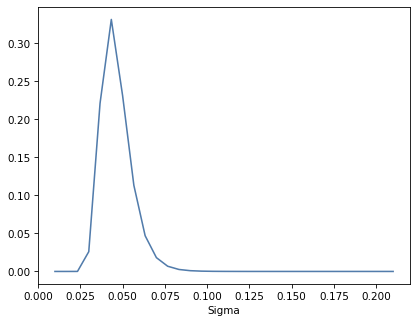
Here’s the posterior distribution for sigma:

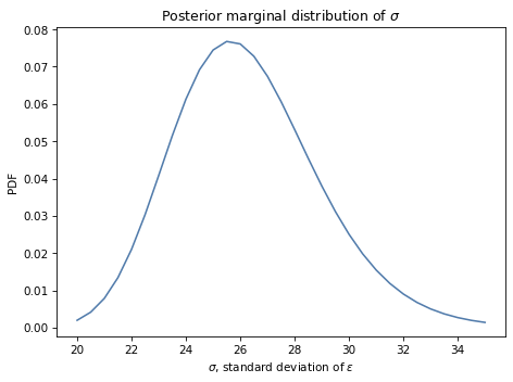
_images/18d3bdf36ae9903d0c61bcf4256b0dc0929fbf4aa4caa9f8d899abefaa3ab113.png

The most likely values for sigma are near 26 inches, which is consistent with our estimate based on the standard deviation of the data.

However, to say whether snowfall is increasing or decreasing, we don’t really care about sigma. It is a “nuisance parameter”, so-called because we have to estimate it as part of the model, but we don’t need it to answer the questions we are interested in.

Nevertheless, it is good to check the marginal distributions to make sure

The location is consistent with our expectations, and
The posterior probabilities are near 0 at the extremes of the range, which indicates that the prior distribution covers all parameters with non-negligible probability.

In this example, the posterior distribution of sigma looks fine.

Here’s the posterior distribution of inter:

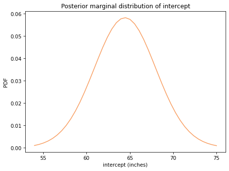
_images/aa89f6dfaa595a9b8213690daa48a4b91af587d81ee8fb38e34bda398382d7db.png

The posterior mean is about 64 inches, which is the expected amount of snow during the year at the midpoint of the range, 1994.

And finally, here’s the posterior distribution of slope:

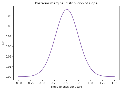
_images/f3b98cd68b7ad121771619d3ad4c437ac7247f6618221ce47119409853c25c97.png

The posterior mean is about 0.51 inches, which is consistent with the estimate we got from least squared regression.

The 90% credible interval is from 0.1 to 0.9, which indicates that our uncertainty about this estimate is pretty high. In fact, there is still a small posterior probability (about 2%) that the slope is negative.

However, it is more likely that my conjecture was wrong: we are actually getting more snow around here than we used to, increasing at a rate of about a half-inch per year, which is substantial. On average, we get an additional 25 inches of snow per year than we did when I was young.

This example shows that with slow-moving trends and noisy data, your instincts can be misleading.

Now, you might suspect that I overestimate the amount of snow when I was young because I enjoyed it, and underestimate it now because I don’t. But you would be mistaken.

During the Blizzard of 1978, we did not have a snowblower and my brother and I had to shovel. My sister got a pass for no good reason. Our driveway was about 60 feet long and three cars wide near the garage. And we had to shovel Mr. Crocker’s driveway, too, for which we were not allowed to accept payment. Furthermore, as I recall it was during this excavation that I accidentally hit my brother with a shovel on the head, and it bled a lot because, you know, scalp wounds.

Anyway, the point is that I don’t think I overestimate the amount of snow when I was young because I have fond memories of it.

Optimization#

The way we computed the likelihood in the previous section was pretty slow. The problem is that we looped through every possible set of parameters in the prior distribution, and there were more than 60,000 of them.

If we can do more work per iteration, and run the loop fewer times, we expect it to go faster.

In order to do that, I’ll unstack the prior distribution:

Show code cell content Hide code cell content

joint3 = prior.unstack()
joint3.head(3)

	Sigma	20.0	20.5	21.0	21.5	22.0	22.5	23.0	23.5	24.0	24.5	...	30.5	31.0	31.5	32.0	32.5	33.0	33.5	34.0	34.5	35.0
Slope	Intercept
-0.5	54.000	0.000015	0.000015	0.000015	0.000015	0.000015	0.000015	0.000015	0.000015	0.000015	0.000015	...	0.000015	0.000015	0.000015	0.000015	0.000015	0.000015	0.000015	0.000015	0.000015	0.000015
	54.525	0.000015	0.000015	0.000015	0.000015	0.000015	0.000015	0.000015	0.000015	0.000015	0.000015	...	0.000015	0.000015	0.000015	0.000015	0.000015	0.000015	0.000015	0.000015	0.000015	0.000015
	55.050	0.000015	0.000015	0.000015	0.000015	0.000015	0.000015	0.000015	0.000015	0.000015	0.000015	...	0.000015	0.000015	0.000015	0.000015	0.000015	0.000015	0.000015	0.000015	0.000015	0.000015

3 rows × 31 columns

The result is a DataFrame with slope and intercept down the rows and sigmas across the columns.

The following is a version of likelihood_regression that takes the joint prior distribution in this form and returns the posterior distribution in the same form.

This version loops through all possible pairs of slope and inter, so the loop runs about 2000 times.

Each time through the loop, it uses a grid mesh to compute the likelihood of the data for all values of sigma. The result is an array with one column for each data point and one row for each value of sigma. Taking the product across the columns (axis=1) yields the probability of the data for each value of sigma, which we assign as a row in likelihood.

We get the same result either way.

But this version is about 25 times faster than the previous version.

This optimization works because many functions in NumPy and SciPy are written in C, so they run fast compared to Python. If you can do more work each time you call these functions, and less time running the loop in Python, your code will often run substantially faster.

In this version of the posterior distribution, slope and inter run down the rows and sigma runs across the columns. So we can use marginal to get the posterior joint distribution of slope and intercept.

Show code cell content Hide code cell content

from utils import marginal

posterior2 = marginal(posterior_opt, 1)
posterior2.head(3)

		probs
Slope	Intercept
-0.5	54.000	1.681717e-07
	54.525	2.268085e-07
	55.050	3.015062e-07

The result is a Pmf with two columns in the index. To plot it, we have to unstack it.

Show code cell content Hide code cell content

joint_posterior = posterior2.unstack().transpose()
joint_posterior.head(3)

Slope	-0.50	-0.46	-0.42	-0.38	-0.34	-0.30	-0.26	-0.22	-0.18	-0.14	...	1.14	1.18	1.22	1.26	1.30	1.34	1.38	1.42	1.46	1.50
Intercept
54.000	1.681717e-07	2.848880e-07	4.744292e-07	7.761707e-07	0.000001	0.000002	0.000003	0.000005	0.000007	0.000010	...	7.116789e-07	4.336070e-07	2.595674e-07	1.527668e-07	8.844849e-08	5.040388e-08	2.828465e-08	1.563589e-08	8.517697e-09	4.573661e-09
54.525	2.268085e-07	3.859703e-07	6.457296e-07	1.061331e-06	0.000002	0.000003	0.000004	0.000006	0.000009	0.000014	...	9.723366e-07	5.896799e-07	3.513780e-07	2.058667e-07	1.186640e-07	6.733065e-08	3.762506e-08	2.071531e-08	1.124098e-08	6.013601e-09
55.050	3.015062e-07	5.153700e-07	8.661024e-07	1.430000e-06	0.000002	0.000004	0.000006	0.000009	0.000013	0.000019	...	1.309030e-06	7.902856e-07	4.688054e-07	2.734522e-07	1.569383e-07	8.867160e-08	4.934762e-08	2.706205e-08	1.462927e-08	7.797870e-09

3 rows × 51 columns

Here’s what it looks like.

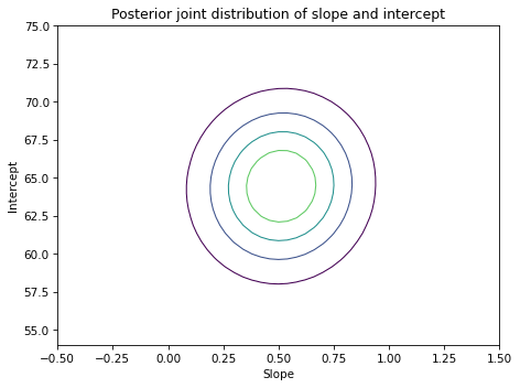
The ovals in the contour plot are aligned with the axes, which indicates that there is no correlation between slope and inter in the posterior distribution, which is what we expect since we centered the values.

In this example, the motivating question is about the slope of the line, so we answered it by looking at the posterior distribution of slope.

In the next example, the motivating question is about prediction, so we’ll use the joint posterior distribution to generate predictive distributions.

Marathon World Record#

For many running events, if you plot the world record pace over time, the result is a remarkably straight line. People, including me, have speculated about possible reasons for this phenomenon.

People have also speculated about when, if ever, the world record time for the marathon will be less than two hours. (Note: In 2019 Eliud Kipchoge ran the marathon distance in under two hours, which is an astonishing achievement that I fully appreciate, but for several reasons it did not count as a world record).

So, as a second example of Bayesian regression, we’ll consider the world record progression for the marathon (for male runners), estimate the parameters of a linear model, and use the model to predict when a runner will break the two-hour barrier.

The following cell downloads a web page from Wikipedia that includes a table of marathon world records, and uses Pandas to put the data in a DataFrame.

If that doesn’t work, I have made a copy of this page available. The following cell downloads and parses it.

The first table is the one we want.

Show code cell content Hide code cell content

table = tables[0]
table.tail(3)

	Time	Name	Nationality	Date	Event/Place	Source	Notes
48	2:02:57	Dennis Kimetto	Kenya	September 28, 2014	Berlin Marathon	IAAF[86][87] ARRS[83]	The ARRS notes Kimetto's extended time as 2:02...
49	2:01:39	Eliud Kipchoge	Kenya	September 16, 2018	Berlin Marathon	IAAF[1]	NaN
50	2:01:09	Eliud Kipchoge	Kenya	September 25, 2022	Berlin Marathon	IAAF[88]	NaN

We can use Pandas to parse the dates. A few of them include notes that cause parsing problems, but the argument errors='coerce' tells Pandas to fill invalid dates with NaT, which is a version of NaN that represents “not a time”.

We can also use Pandas to parse the record times.

And convert the times to paces in miles per hour.

The following function plots the results.

Here’s what the results look like. The dashed line shows the speed required for a two-hour marathon, 13.1 miles per hour.

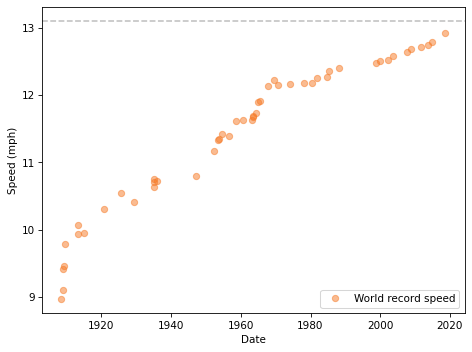
It’s not a perfectly straight line. In the early years of the marathon, the record speed increased quickly; since about 1970, it has been increasing more slowly.

For our analysis, let’s focus on the recent progression, starting in 1970.

Show code cell content Hide code cell content

recent = table['date'] > pd.to_datetime('1970')
data = table.loc[recent].copy()
data.head()

	Time	Name	Nationality	Date	Event/Place	Source	Notes	date	time	y
32	2:09:28.8	Ron Hill	United Kingdom	July 23, 1970	Edinburgh, Scotland	ARRS[9]	NaN	1970-07-23	0 days 02:09:28.800000	12.140871
33	2:09:12	Ian Thompson	United Kingdom	January 31, 1974	Christchurch, New Zealand	ARRS[9]	NaN	1974-01-31	0 days 02:09:12	12.167183
34	2:09:05.6	Shigeru So	Japan	February 5, 1978	Beppu-Ōita Marathon	ARRS[9]	NaN	1978-02-05	0 days 02:09:05.600000	12.177236
35	2:09:01	Gerard Nijboer	Netherlands	April 26, 1980	Amsterdam Marathon	ARRS[9]	NaN	1980-04-26	0 days 02:09:01	12.184472
36	2:08:18	Robert De Castella	Australia	December 6, 1981	Fukuoka Marathon	IAAF,[53] ARRS[9]	NaN	1981-12-06	0 days 02:08:18	12.252533

In the notebook for this chapter, you can see how I loaded and cleaned the data. The result is a DataFrame that contains the following columns (and additional information we won’t use):

date, which is a Pandas Timestamp representing the date when the world record was broken, and
speed, which records the record-breaking pace in mph.

Here’s what the results look like, starting in 1970:

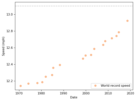
_images/e0e47c76527482395e93a96135d115eca888e0ad44e1dea1a7ba82dfd6d4b5d2.png

The data points fall approximately on a line, although it’s possible that the slope is increasing.

To prepare the data for regression, I’ll subtract away the approximate midpoint of the time interval, 1995.

offset = pd.to_datetime('1995')
timedelta = table['date'] - offset

When we subtract two Timestamp objects, the result is a “time delta”, which we can convert to seconds and then to years.

data['x'] = timedelta.dt.total_seconds() / 3600 / 24 / 365.24

As in the previous example, I’ll use least squares regression to compute point estimates for the parameters, which will help with choosing priors.

import statsmodels.formula.api as smf

formula = 'y ~ x'
results = smf.ols(formula, data=data).fit()
results.params

Intercept    12.464040
x             0.015931
dtype: float64

The estimated intercept is about 12.5 mph, which is the interpolated world record pace for 1995. The estimated slope is about 0.015 mph per year, which is the rate the world record pace is increasing, according to the model.

Again, we can use the standard deviation of the residuals as a point estimate for sigma.

results.resid.std()

0.04419653543387639

These parameters give us a good idea where we should put the prior distributions.

The Priors#

Here are the prior distributions I chose for slope, intercept, and sigma.

qs = np.linspace(0.012, 0.018, 51)
prior_slope = make_uniform(qs, 'Slope')

qs = np.linspace(12.4, 12.5, 41)
prior_inter = make_uniform(qs, 'Intercept')

qs = np.linspace(0.01, 0.21, 31)
prior_sigma = make_uniform(qs, 'Sigma')

And here’s the joint prior distribution.

prior = make_joint3(prior_slope, prior_inter, prior_sigma)
prior.head()

			probs
Slope	Intercept	Sigma
0.012	12.4	0.010000	0.000015
		0.016667	0.000015
		0.023333	0.000015

Now we can compute likelihoods as in the previous example:

xs = data['x']
ys = data['y']
likelihood = prior.copy()

for slope, inter, sigma in prior.index:
    expected = slope * xs + inter
    resid = ys - expected
    densities = norm.pdf(resid, 0, sigma)
    likelihood[slope, inter, sigma] = densities.prod()

Now we can do the update in the usual way.

posterior = prior * likelihood
posterior.normalize()

And unpack the marginals:

posterior_slope = posterior.marginal(0)
posterior_inter = posterior.marginal(1)
posterior_sigma = posterior.marginal(2)

Here’s the posterior distribution of inter:

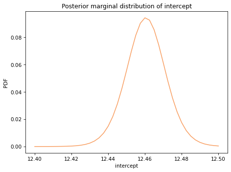
_images/0672371f2c001a21e11016942fe04bcb4761581494d3b6bec0bb5d585b516904.png

The posterior mean is about 12.5 mph, which is the world record marathon pace the model predicts for the midpoint of the date range, 1994.

And here’s the posterior distribution of slope.

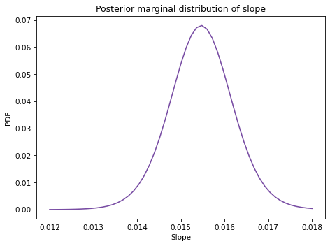
_images/7109d0d15b11012912c742b75e4e4c39cd5dfb2818b8a301ce029d65ac800228.png

The posterior mean is about 0.015 mph per year, or 0.15 mph per decade.

That’s interesting, but it doesn’t answer the question we’re interested in: When will there be a two-hour marathon? To answer that, we have to make predictions.

Prediction#

To generate predictions, I’ll draw a sample from the posterior distribution of parameters, then use the regression equation to combine the parameters with the data.

Pmf provides choice, which we can use to draw a random sample with replacement, using the posterior probabilities as weights.

sample = posterior.choice(101)

The result is an array of tuples. Looping through the sample, we can use the regression equation to generate predictions for a range of xs.

xs = np.arange(-25, 50, 2)
pred = np.empty((len(sample), len(xs)))

for i, (slope, inter, sigma) in enumerate(sample):
    epsilon = norm(0, sigma).rvs(len(xs))
    pred[i] = inter + slope * xs + epsilon

Each prediction is an array with the same length as xs, which I store as a row in pred. So the result has one row for each sample and one column for each value of x.

We can use percentile to compute the 5th, 50th, and 95th percentiles in each column.

low, median, high = np.percentile(pred, [5, 50, 95], axis=0)

To show the results, I’ll plot the median of the predictions as a line and the 90% credible interval as a shaded area.

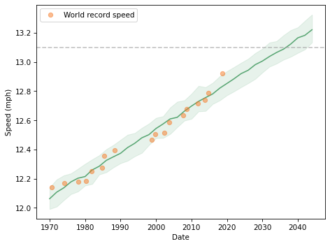
_images/da26aaa0faaca034b92e93a2aa91612ff8cef66bda7d869e32bd0f48698d039a.png

The dashed line shows the two-hour marathon pace, which is 13.1 miles per hour. Visually we can estimate that the prediction line hits the target pace between 2030 and 2040.

To make this more precise, we can use interpolation to see when the predictions cross the finish line. SciPy provides interp1d, which does linear interpolation by default.

from scipy.interpolate import interp1d

future = np.array([interp1d(high, xs)(13.1),
                   interp1d(median, xs)(13.1),
                   interp1d(low, xs)(13.1)])

Show code cell content Hide code cell content

dts = pd.to_timedelta(future*365.24, unit='day') + offset
pd.DataFrame(dict(datetime=dts),
             index=['early', 'median', 'late'])

	datetime
early	2028-03-24 16:47:21.722121600
median	2035-03-10 14:59:51.082915200
late	2040-12-29 22:53:36.679804800

The median prediction is 2036, with a 90% credible interval from 2032 to 2043. So there is about a 5% chance we’ll see a two-hour marathon before 2032.

Summary#

This chapter introduces Bayesian regression, which is based on the same model as least squares regression; the difference is that it produces a posterior distribution for the parameters rather than point estimates.

In the first example, we looked at changes in snowfall in Norfolk County, Massachusetts, and concluded that we get more snowfall now than when I was young, contrary to my expectation.

In the second example, we looked at the progression of world record pace for the men’s marathon, computed the joint posterior distribution of the regression parameters, and used it to generate predictions for the next 20 years.

These examples have three parameters, so it takes a little longer to compute the likelihood of the data. With more than three parameters, it becomes impractical to use grid algorithms.

In the next few chapters, we’ll explore other algorithms that reduce the amount of computation we need to do a Bayesian update, which makes it possible to use models with more parameters.

But first, you might want to work on these exercises.

Exercises#

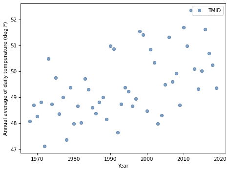
Exercise: I am under the impression that it is warmer around here than it used to be. In this exercise, you can put my conjecture to the test.

We’ll use the same dataset we used to model snowfall; it also includes daily low and high temperatures in Norfolk County, Massachusetts during my lifetime.

Here’s the data.

Show code cell content Hide code cell content

df = pd.read_csv('2239075.csv', parse_dates=[2])
df.head(3)

	STATION	NAME	DATE	PRCP	TMAX	TMIN	TOBS	WESD	WT01	WT03	WT04	WT05	WT06	WT08	WT09	WT11	WT16	WT18
0	USC00190736	BLUE HILL COOP, MA US	1967-05-11	0.43	57	36.0	NaN	NaN	NaN	NaN	NaN	NaN	NaN	NaN	NaN	NaN	NaN	NaN
1	USC00190736	BLUE HILL COOP, MA US	1967-05-12	0.00	58	39.0	NaN	NaN	NaN	NaN	NaN	NaN	NaN	NaN	NaN	NaN	NaN	NaN
2	USC00190736	BLUE HILL COOP, MA US	1967-05-13	0.00	64	38.0	NaN	NaN	NaN	NaN	NaN	NaN	NaN	NaN	NaN	NaN	NaN	NaN

Again, I’ll create a column that contains the year part of the dates.

This dataset includes TMIN and TMAX, which are the daily low and high temperatures in degrees F. I’ll create a new column with the daily midpoint of the low and high temperatures.

Now we can group by year and compute the mean of these daily temperatures.

Again, I’ll drop the first and last years, which are incomplete.

Here’s what the time series looks like.

As we did with the snow data, I’ll convert the Series to a DataFrame to prepare it for regression.

Show code cell content Hide code cell content

data = complete.reset_index()
data.head()

	YEAR	TMID
0	1968	48.071038
1	1969	48.687671
2	1970	48.258904
3	1971	48.804110
4	1972	47.112022

Now we can use StatsModels to estimate the parameters.

And compute the standard deviation of the parameters.

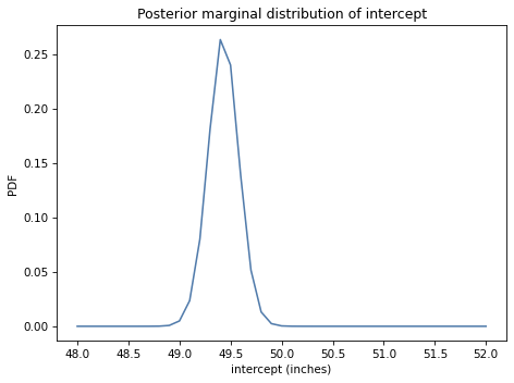
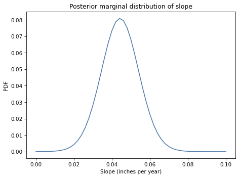
According to the least squares regression model, annual average temperature is increasing by about 0.044 degrees F per year.

To quantify the uncertainty of these parameters and generate predictions for the future, we can use Bayesian regression.

Use StatsModels to generate point estimates for the regression parameters.
Choose priors for slope, intercept, and sigma based on these estimates, and use make_joint3 to make a joint prior distribution.
Compute the likelihood of the data and compute the posterior distribution of the parameters.
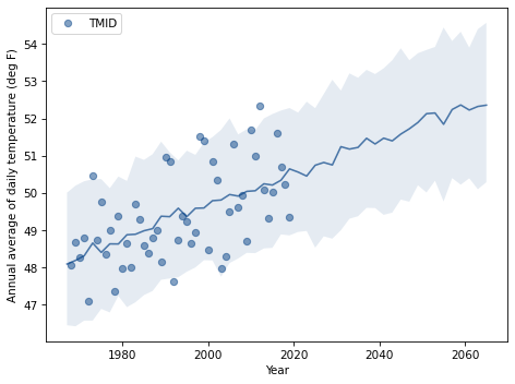
Extract the posterior distribution of slope. How confident are we that temperature is increasing?
Draw a sample of parameters from the posterior distribution and use it to generate predictions up to 2067.
Plot the median of the predictions and a 90% credible interval along with the observed data.

Does the model fit the data well? How much do we expect annual average temperatures to increase over my (expected) lifetime?

Show code cell content Hide code cell content

# Solution

prior = make_joint3(prior_slope, prior_inter, prior_sigma)
prior.head()

			probs
Slope	Intercept	Sigma
0.0	48.0	0.50	0.000015
		0.55	0.000015
		0.60	0.000015

Regression

Contents

Regression#

More Snow?#

Regression Model#

Least Squares Regression#

Priors#

Likelihood#

The Update#

Optimization#

Marathon World Record#

The Priors#

Prediction#

Summary#

Exercises#