You can order print and ebook versions of Think Bayes 2e from Bookshop.org and Amazon.
Bayesian Dice#
Click here to run this notebook on Colab
I’ve been enjoying Aubrey Clayton’s new book Bernoulli’s Fallacy. Chapter 1, which is about the historical development of competing definitions of probability, is worth the price of admission alone.
One of the examples in the first chapter is a simplified version of a problem posed by Thomas Bayes. The original version, which I wrote about here, involves a billiards (pool) table; Clayton’s version uses dice:
Your friend rolls a six-sided die and secretly records the outcome; this number becomes the target T. You then put on a blindfold and roll the same six-sided die over and over. You’re unable to see how it lands, so each time your friend […] tells you only whether the number you just rolled was greater than, equal to, or less than T.
Suppose in one round of the game we had this sequence of outcomes, with G representing a greater roll, L a lesser roll, and E an equal roll:
G, G, L, E, L, L, L, E, G, L
Based on this data, what is the posterior distribution of T?
Computing likelihoods#
There are two parts of my solution; computing the likelihood of the data under each hypothesis and then using those likelihoods to compute the posterior distribution of T.
To compute the likelihoods, I’ll demonstrate one of my favorite idioms, using a meshgrid to apply an operation, like >, to all pairs of values from two sequences.
In this case, the sequences are
hypos: The hypothetical values of T, andoutcomes: possible outcomes each time we roll the dice
hypos = [1,2,3,4,5,6]
outcomes = [1,2,3,4,5,6]
If we compute a meshgrid of outcomes and hypos, the result is two arrays.
import numpy as np

O, H = np.meshgrid(outcomes, hypos)
The first contains the possible outcomes repeated down the columns.
O
array([[1, 2, 3, 4, 5, 6],
       [1, 2, 3, 4, 5, 6],
       [1, 2, 3, 4, 5, 6],
       [1, 2, 3, 4, 5, 6],
       [1, 2, 3, 4, 5, 6],
       [1, 2, 3, 4, 5, 6]])
The second contains the hypotheses repeated across the rows.
H
array([[1, 1, 1, 1, 1, 1],
       [2, 2, 2, 2, 2, 2],
       [3, 3, 3, 3, 3, 3],
       [4, 4, 4, 4, 4, 4],
       [5, 5, 5, 5, 5, 5],
       [6, 6, 6, 6, 6, 6]])
If we apply an operator like >, the result is a Boolean array.
O > H
array([[False,  True,  True,  True,  True,  True],
       [False, False,  True,  True,  True,  True],
       [False, False, False,  True,  True,  True],
       [False, False, False, False,  True,  True],
       [False, False, False, False, False,  True],
       [False, False, False, False, False, False]])
Now we can use mean with axis=1 to compute the fraction of True values in each row.
(O > H).mean(axis=1)
array([0.83333333, 0.66666667, 0.5       , 0.33333333, 0.16666667,
       0.        ])
The result is the probability that the outcome is greater than T, for each hypothetical value of T.
I’ll name this array gt:
gt = (O > H).mean(axis=1)
gt
array([0.83333333, 0.66666667, 0.5       , 0.33333333, 0.16666667,
       0.        ])
The first element of the array is 5/6, which indicates that if T is 1, the probability of exceeding it is 5/6. The second element is 2/3, which indicates that if T is 2, the probability of exceeding it is 2/3. And do on.
Now we can compute the corresponding arrays for less than and equal.
lt = (O < H).mean(axis=1)
lt
array([0.        , 0.16666667, 0.33333333, 0.5       , 0.66666667,
       0.83333333])
eq = (O == H).mean(axis=1)
eq
array([0.16666667, 0.16666667, 0.16666667, 0.16666667, 0.16666667,
       0.16666667])
In the next section, we’ll use these arrays to do a Bayesian update.
The Update#
In this example, computing the likelihoods was the hard part. The Bayesian update is easy.
Since T was chosen by rolling a fair die, the prior distribution for T is uniform.
I’ll use a Pandas Series to represent it.
import pandas as pd

pmf = pd.Series(1/6, hypos)
pmf
1    0.166667
2    0.166667
3    0.166667
4    0.166667
5    0.166667
6    0.166667
dtype: float64
Now here’s the sequence of data, encoded using the likelihoods we computed in the previous section.
data = [gt, gt, lt, eq, lt, lt, lt, eq, gt, lt]
The following loop updates the prior distribution by multiplying by each of the likelihoods.
for datum in data:
    pmf *= datum
Finally, we normalize the posterior.
pmf /= pmf.sum()
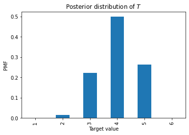
pmf
1    0.000000
2    0.016427
3    0.221766
4    0.498973
5    0.262834
6    0.000000
dtype: float64
Here’s what it looks like.
pmf.plot.bar(xlabel='Target value',
             ylabel='PMF',
             title='Posterior distribution of $T$');
As an aside, you might have noticed that the values in eq are all the same.
So when the value we roll is equal to \(T\), we don’t get any new information about T.
We could leave the instances of eq out of the data, and we would get the same answer.