How Many Typos?

How Many Typos?#

When I started work at Brilliant a couple of weeks ago, I learned that one of my new colleagues, Michelle McSweeney, just published a book called OK, which is all about the word OK.

As we discussed the joys and miseries of publishing, Michelle mentioned that she had found a typo in the book after publication. So naturally I took it as a challenge to find the typo. While I was searching, I enjoyed the book very much. If you are interested in etymology, linguistics, and history, I recommend it!

As it turned out, I found exactly one typo. When I told Michelle, she asked me nervously which page it was on. Page 17. She looked disappointed – that was not the same typo she found.

Now, for people who like Bayesian statistics, this scenario raises some questions:

After our conversation, how many additional typos should we expect there to be?
If she and I had found the same typo, instead of different ones, how many typos would we expect?

As it happens, I used a similar scenario as an example in Think Bayes. This notebook is based on the code I presented there. If there’s anything here that’s not clear, you could read the chapter for more details.

You can also click here to run this notebook on Colab.

A Warm-up Problem#

Starting with a simple version of the problem, let’s assume that we know p0 and p1, which are the probabilities, respectively, that the first and second readers find any given typo.

For example, let’s assume that Michelle has a 66% chance of finding a typo and I have a 50% chance.

p0, p1 = 0.66, 0.5

With these assumptions, we can compute an array that contains (in order) the probability that neither of us find a typo, the probability that only the second reader does, the probability that the first reader does, and the probability that we both do.

def compute_probs(p0, p1):
    """Computes the probability for each of 4 categories."""
    q0 = 1-p0
    q1 = 1-p1
    return [q0*q1, q0*p1, p0*q1, p0*p1]

y = compute_probs(p0, p1)
y

[0.16999999999999998, 0.16999999999999998, 0.33, 0.33]

With the assumed probabilities, there is a 33% chance that we both find a typo and a 17% chance that neither of us do.

The Prior#

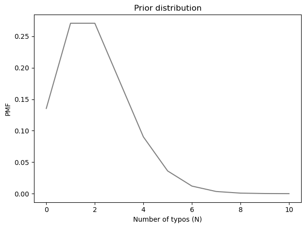
Next we need to choose a prior for the total number of typos. I’ll use a Poisson distribution, which is a reasonable default for values that are counts. And I’ll set the mean to 2, which means that before either of us read the book, we would have expected about two typos.

from utils import make_poisson_pmf

qs = np.arange(0, 11) 
lam = 2
prior_N = make_poisson_pmf(lam, qs)
prior_N.index.name = 'N'
prior_N.mean()

1.9999236196641172

Here’s what the prior looks like.

_images/77726d32755a0911144b37af88df7d5b01545b8f0092aaa4754562c4c6801e50.png

The Update (Simple Version)#

To represent the data, I’ll create these variables:

k10: the number of typos found by the first reader but not the second
k01: the number of typos found by the second reader but not the first
k11: the number of typos found by both readers

k10 = 1
k01 = 1
k11 = 0

I’ll put the data in an array, with 0 as a place-keeper for the unknown value k00, which is the number of typos neither of us found.

data = np.array([0, k01, k10, k11])

Now we can use the multinomial distribution to compute the likelihood of the data for each hypothetical value of N (assuming for now that the probabilities in y are known).

from scipy.stats import multinomial

likelihood = prior_N.copy()
observed = data.sum()
x = data.copy()

for N in prior_N.qs:
    x[0] = N - observed
    likelihood[N] = multinomial.pmf(x, N, y)

We can compute the posterior in the usual way.

posterior_N = prior_N * likelihood
posterior_N.normalize()

0.0426675416210306

And here’s what it looks like.

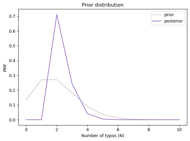
_images/e9548bb3eda665fa8cc1684da08ffe2df31f833e2ec55e22d0f4c6a08b185931.png

The most likely value is 2, and the posterior mean is about 2.3, just a little higher than the prior mean.

But remember that this is based on the assumption that we know p0 and p1. In reality, they are unknown, but we can estimate them from the data.

Three-Parameter Model#

What we need is a model with three parameters: N, p0, and p1. We’ll use prior_N again for the prior distribution of N, and here are the priors for p0 and p1:

from empiricaldist import Pmf
from scipy.stats import beta as beta_dist

def make_beta(qs, alpha, beta, name=""):
    ps = beta_dist.pdf(qs, alpha, beta)
    pmf = Pmf(ps, qs)
    pmf.normalize()
    pmf.index.name = name
    return pmf

qs = np.linspace(0, 1, num=51)
prior_p0 = make_beta(qs, 3, 2, name='p0')
prior_p1 = make_beta(qs, 2, 2, name='p1')

prior_p0.plot()
prior_p1.plot()

decorate(xlabel='Probability of finding a typo',
         ylabel='PMF',
         title='Prior distributions')

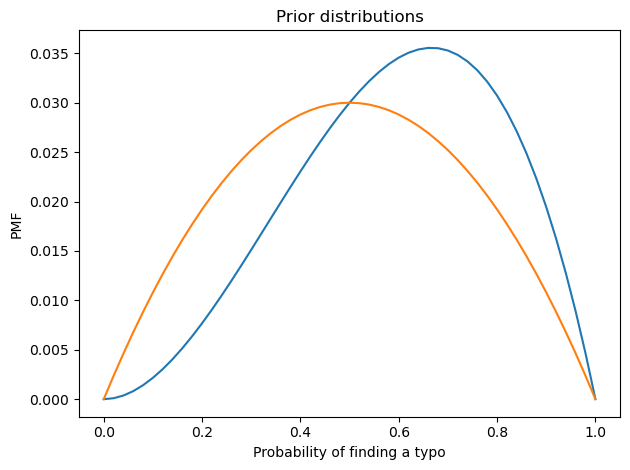
_images/7e0d1a057533e834e15cc2de09bb543b9108cd175ccce907df9079147b09c1be.png

I used beta distributions to construct weakly informative priors for p0 and p1, with means 0.66 and 0.5 respectively.

The Joint Prior#

Now we have to assemble the marginal priors into a joint distribution. I’ll start by putting the first two into a DataFrame.

from utils import make_joint

joint2 = make_joint(prior_p0, prior_N)
joint2.shape

(11, 51)

Now I’ll stack them and put the result in a Pmf.

joint2_pmf = Pmf(joint2.stack())
joint2_pmf.head(3)

		probs
N	p0
0	0.00	0.000000
	0.02	0.000013
	0.04	0.000050

We can use make_joint again to add in the third parameter.

joint3 = make_joint(prior_p1, joint2_pmf)
joint3.shape

(561, 51)

The result is a DataFrame with values of N and p0 in a MultiIndex that goes down the rows and values of p1 in an index that goes across the columns.

joint3.head(3)

	p1	0.00	0.02	0.04	0.06	0.08	0.10	0.12	0.14	0.16	0.18	...	0.82	0.84	0.86	0.88	0.90	0.92	0.94	0.96	0.98	1.00
N	p0
0	0.00	0.0	0.000000e+00	0.000000e+00	0.000000e+00	0.000000e+00	0.000000e+00	0.000000e+00	0.000000e+00	0.000000e+00	0.000000e+00	...	0.000000e+00	0.000000e+00	0.000000e+00	0.000000e+00	0.000000e+00	0.000000e+00	0.000000e+00	0.000000e+00	0.000000e+00	0.0
	0.02	0.0	2.997069e-08	5.871809e-08	8.624220e-08	1.125430e-07	1.376205e-07	1.614748e-07	1.841057e-07	2.055133e-07	2.256977e-07	...	2.256977e-07	2.055133e-07	1.841057e-07	1.614748e-07	1.376205e-07	1.125430e-07	8.624220e-08	5.871809e-08	2.997069e-08	0.0
	0.04	0.0	1.174362e-07	2.300791e-07	3.379286e-07	4.409848e-07	5.392478e-07	6.327174e-07	7.213937e-07	8.052767e-07	8.843664e-07	...	8.843664e-07	8.052767e-07	7.213937e-07	6.327174e-07	5.392478e-07	4.409848e-07	3.379286e-07	2.300791e-07	1.174362e-07	0.0

3 rows × 51 columns

Now I’ll apply stack again:

joint3_pmf = Pmf(joint3.stack())
joint3_pmf.head(3)

			probs
N	p0	p1
0	0.0	0.00	0.0
		0.02	0.0
		0.04	0.0

The result is a Pmf with a three-column MultiIndex containing all possible triplets of parameters.

The number of rows is the product of the number of values in all three priors:

joint3_pmf.shape

(28611,)

That’s still small enough to be practical, but it will take longer to compute the likelihoods than in the previous example.

The Update (Three-Parameter Version)#

Here’s the loop that computes the likelihoods. It’s similar to the one in the previous section, except that y is no longer constant; we compute it each time through the loop from hypothetical values of p0 and p1.

likelihood = joint3_pmf.copy()
observed = data.sum()
x = data.copy()

for N, p0, p1 in joint3_pmf.index:
    x[0] = N - observed
    y = compute_probs(p0, p1)
    likelihood[N, p0, p1] = multinomial.pmf(x, N, y)

/home/downey/miniconda3/envs/ThinkBayes2/lib/python3.10/site-packages/scipy/stats/_multivariate.py:3190: RuntimeWarning: invalid value encountered in subtract
  return gammaln(n+1) + np.sum(xlogy(x, p) - gammaln(x+1), axis=-1)

We can compute the posterior in the usual way.

posterior_pmf = joint3_pmf * likelihood
posterior_pmf.normalize()

0.03437554251769621

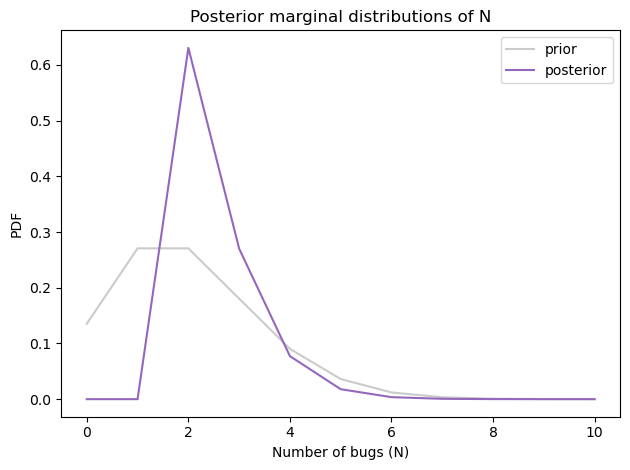
Here’s the posterior marginal distribution N.

posterior_N = posterior_pmf.marginal(0)

prior_N.plot(color='C7', alpha=0.4, label='prior')
posterior_N.plot(color='C4', label='posterior')

decorate(xlabel='Number of bugs (N)',
         ylabel='PDF',
         title='Posterior marginal distributions of N')

_images/521e5ac757cf28dc37bb176c71850b5773b74cdf68d0ea45e694a617bac42457.png

To compute the probability that there is at least one undiscovered typo, we can convert the posterior distribution to a survival function (complementary CDF):

posterior_N.make_surv()[observed]

0.369576444173048

The probability is about 37% that there’s another typo – so that’s good news!

The posterior mean is about 2.5, which is a little higher than what we got with the simple model.

posterior_N.mean()

2.4963989774563107

Apparently our uncertainty about p0 and p1 leaves open the possibility that there are more typos and we are not very good at finding them. Here’s what the posterior distributions look like for p0 and p1.

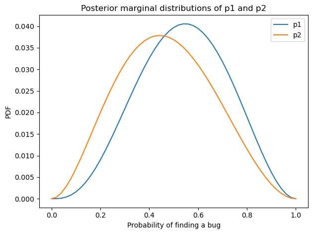
_images/b1402fb19dc1e3caa863266c73b6723a8334d075a54cad8f228d32265e115cc6.png

With so little data, the posterior distributions are still quite wide, but the posterior means are a little smaller than the priors.

posterior_p1.mean(), posterior_p1.credible_interval(0.9)

(0.5383375553393667, array([0.24, 0.82]))

posterior_p2.mean(), posterior_p2.credible_interval(0.9)

(0.46718395159883724, array([0.16, 0.78]))

The fact that Michelle and I found only two typos is weak evidence that we are not as good at finding them as the priors implied.

At this point, we’ve answered the first question: given that Michelle and I found different bugs, the expected value for the number of remaining typos is about 0.5.

In the counterfactual case, if we had found the same typo, we would represent the data like this:

k10 = 0
k01 = 0
k11 = 1

If we run the analysis with this data, we find:

The expected number of remaining typos is about 0.3 (compared to 0.5),
there would be only a 25% chance that there is at least one undiscovered typo, and
we would conclude that Michelle and I are slightly better at finding typos.

This notebook is based on this chapter of Think Bayes, Second Edition.

License: Attribution-NonCommercial-ShareAlike 4.0 International (CC BY-NC-SA 4.0)