In Search of the Fourth Wave

In Search of the Fourth Wave#

Click here to run this notebook on Colab.

Allen Downey#

Olin College

DSP Online Conference

When I was working on Think DSP, I encountered a small mystery.

As you might know:

A sawtooth wave contains harmonics at integer multiples of the fundamental frequency, and
Their amplitudes drop off in proportion to \(1/f\).

A square wave contains only odd multiples of the fundamental, but
They also drop off like \(1/f\).

A triangle wave also contains only odd multiples,
But they drop off like \(1/f^2\).

Which suggests that there’s a simple waveform that

Contains all integer multiples (like a sawtooth) and
Drops off like \(1/f^2\) (like a triangle wave).

Let’s find out what it is.

In this talk, I’ll

Suggest four ways we can find the mysterious fourth wave.
Demonstrate using tools from SciPy, NumPy and Pandas, and

And a tour of DSP and the topics in Think DSP.

I’m a professor of Computer Science at Olin College.

Author of Think Python, Think Bayes, and Think DSP.

And Probably Overthinking It, a blog about Bayesian probability and statistics.

Web page: allendowney.com

Twitter: @allendowney

This talk is a Jupyter notebook.

You can read it here.

And run it here.

Here are the libraries we’ll use.

import numpy as np
import pandas as pd
import matplotlib.pyplot as plt

And a convenience function for decorating figures.

def decorate(**options):
    """Decorate the current axes.

    Call decorate with keyword arguments like

    decorate(title='Title',
             xlabel='x',
             ylabel='y')

    The keyword arguments can be any of the axis properties

    https://matplotlib.org/api/axes_api.html

    In addition, you can use `legend=False` to suppress the legend.

    And you can use `loc` to indicate the location of the legend
    (the default value is 'best')
    """
    plt.gca().set(**options)
    plt.tight_layout()

def legend(**options):
    """Draws a legend only if there is at least one labeled item.

    options are passed to plt.legend()
    https://matplotlib.org/api/_as_gen/matplotlib.plt.legend.html

    """
    ax = plt.gca()
    handles, labels = ax.get_legend_handles_labels()
    if handles:
        ax.legend(handles, labels, **options)

Basic waveforms#

We’ll start with the basic waveforms:

sawtooth,
triangle, and
square.

Sampled at CD audio frame rate.

framerate = 44100        # samples per second
dt = 1 / framerate       # seconds per sample

At equally-spaced times from 0 to duration.

duration = 0.005                    # seconds
ts = np.arange(0, duration, dt)     # seconds

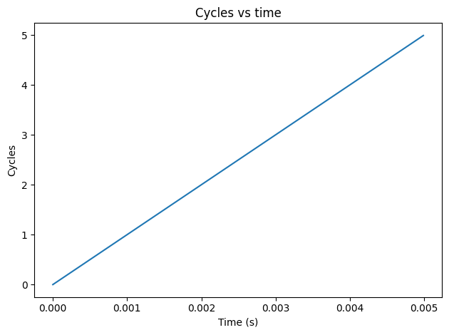
We’ll work with signals at 1000 Hz.

The number of complete cycles is \(f t\).

freq = 1000              # cycles per second (Hz)
cycles = freq * ts       # cycles

In 0.005 seconds, a 1000 Hz signal completes 5 cycles.

np.max(cycles)

np.float64(4.988662131519274)

plt.plot(ts, cycles)

decorate(xlabel='Time (s)',
         ylabel='Cycles',
         title='Cycles vs time')

_images/3691aacce6f20925bab65e4c6de963521adbc4cb016b6f2820262d27e0517619.png

wrap uses modf to compute the fraction part of the number of cycles.

def wrap(cycles):
    frac, _ = np.modf(cycles)
    return frac

If we apply wrap to cycles, the result is a sawtooth wave.

I subtract off 0.5 so the mean of the signal is 0.

ys = wrap(cycles) - 0.5
ys.mean()

np.float64(0.003380839515293344)

Here’s what it looks like.

plt.plot(ts, ys)

decorate(xlabel='Time (s)',
         ylabel='Amplitude',
         title='Sawtooth Wave')

If we take the absolute value of ys, the result is a triangle wave.

plt.plot(ts, np.abs(ys))

decorate(xlabel='Time (s)',
         ylabel='Amplitude',
         title='Triangle wave')

And if we take just the sign of ys, the result is a square wave.

plt.plot(ts, np.sign(ys))

decorate(xlabel='Time (s)',
         ylabel='Amplitude',
         title='Square wave')

Think of abs as magnitude and sign as direction

The triangle is the magnitude of a sawtooth.
The square wave is the direction of a sawtooth.

One function to make them all#

make_wave contains the parts these waves have in common.

def make_wave(func, duration, freq):
    """Make a signal.
    
    func: function that takes cycles and computes ys
    duration: length of the wave in time
    """
    ts = np.arange(0, duration, dt)
    cycles = freq * ts    
    ys = func(cycles)
    
    ys = unbias(normalize(ys))
    series = pd.Series(ys, ts)
    return series

normalize scales the wave between 0 and 1,

unbias shifts it so the mean is 0.

def normalize(ys):
    low, high = np.min(ys), np.max(ys)
    return (ys - low) / (high - low)

def unbias(ys):
    return ys - ys.mean()

Why use a Series?

Series is like two arrays:

An index, and
Corresponding value.

Natural representation of correspondence:

From time to amplitude.
From frequency to complex amplitude.

We’ll use plot_wave to plot a short segment of a wave.

def plot_wave(wave, title=''):
    segment = wave[0:0.01]
    segment.plot()
    decorate(xlabel='Time (s)',
             ylabel='Amplitude',
             title=title)

Now we can define sawtooth_func to compute the sawtooth wave.

def sawtooth_func(cycles):
    ys = wrap(cycles) - 0.5
    return ys

And pass it as an argument to make_wave:

sawtooth_wave = make_wave(sawtooth_func, duration=0.01, freq=500)
plot_wave(sawtooth_wave, title='Sawtooth wave')

Same with triangle_func.

def triangle_func(cycles):
    ys = wrap(cycles) - 0.5
    return np.abs(ys)

triangle_wave = make_wave(triangle_func, duration=0.01, freq=500)
plot_wave(triangle_wave, title='Triangle wave')

And square_func.

def square_func(cycles):
    ys = wrap(cycles) - 0.5
    return np.sign(ys)

square_wave = make_wave(square_func, duration=0.01, freq=500)
plot_wave(square_wave, title='Square wave')

Spectrum#

Now let’s see what the spectrums look like for these waves.

def make_spectrum(wave):
    n = len(wave)
    hs = np.fft.rfft(wave)         # amplitudes
    fs = np.fft.rfftfreq(n, dt)    # frequencies

    series = pd.Series(hs, fs)
    return series

make_spectrum uses NumPy to compute the real FFT of the wave:

hs contains the complex amplitudes, and
fs contains the corresponding frequencies.

Pandas Series represents correspondence between frequencies and complex amplitudes.

Use abs to compute magnitude of complex amplitudes and plot them as a function of fs:

def plot_spectrum(spectrum, title=''):
    spectrum.abs().plot()
    decorate(xlabel='Frequency (Hz)',
             ylabel='Magnitude',
             title=title)

I’ll use a sinusoid to test make_spectrum.

def sinusoid_func(cycles):
    return np.cos(2 * np.pi * cycles)

Now we can use make_wave to make a sinusoid.

sinusoid_wave = make_wave(sinusoid_func, duration=0.5, freq=freq)

And make_spectrum to compute its spectrum.

sinusoid_spectrum = make_spectrum(sinusoid_wave)
plot_spectrum(sinusoid_spectrum, 
              title='Spectrum of a sinusoid wave')

A sinusoid only contains one frequency component.

As contrasted with the spectrum of a sawtooth wave, which looks like this.

sawtooth_wave = make_wave(sawtooth_func, duration=0.5, freq=freq)
sawtooth_spectrum = make_spectrum(sawtooth_wave)
plot_spectrum(sawtooth_spectrum, 
              title='Spectrum of a sawtooth wave')

The largest magnitude is at 1000 Hz, but the signal also contains components at every integer multiple of the fundamental frequency.

Here’s the spectrum of a square wave with the same fundamental frequency.

square_wave = make_wave(square_func, duration=0.5, freq=freq)
square_spectrum = make_spectrum(square_wave)
plot_spectrum(square_spectrum, 
              title='Spectrum of a square wave')

The spectrum of the square wave has only odd harmonics.

triangle_wave = make_wave(triangle_func, duration=0.5, freq=freq)
triangle_spectrum = make_spectrum(triangle_wave)
plot_spectrum(triangle_spectrum, 
              title='Spectrum of a triangle wave')

The spectrum of the triangle wave has odd harmonics only.

But they drop off more quickly.

Sound#

make_audio makes an IPython Audio object we can use to play a wave.

from IPython.display import Audio

def make_audio(wave):
    """Makes an IPython Audio object.
    """
    return Audio(data=wave, rate=framerate)

Dropping to 500 Hz to spare your ears.

freq = 500

sinusoid_wave = make_wave(sinusoid_func, duration=0.5, freq=freq)
make_audio(sinusoid_wave)

triangle_wave = make_wave(triangle_func, duration=0.5, freq=freq)
make_audio(triangle_wave)

sawtooth_wave = make_wave(sawtooth_func, duration=0.5, freq=freq)
make_audio(sawtooth_wave)

square_wave = make_wave(square_func, duration=0.5, freq=freq)
make_audio(square_wave)

Dropoff#

Let’s see how the spectrums depend on \(f\).

def plot_over_f(spectrum, freq, exponent):
    fs = spectrum.index
    hs = 1 / fs**exponent

    over_f = pd.Series(hs, fs)
    over_f[fs<freq] = np.nan
    over_f *= np.abs(spectrum[freq]) / over_f[freq]
    over_f.plot(color='gray')

freq = 500

sawtooth_wave = make_wave(func=sawtooth_func, 
                          duration=0.5, freq=freq)
sawtooth_spectrum = make_spectrum(sawtooth_wave)

plot_over_f(sawtooth_spectrum, freq, 1)
plot_spectrum(sawtooth_spectrum, 
              title='Spectrum of a sawtooth wave')

square_wave = make_wave(func=square_func, 
                        duration=0.5, freq=freq)
square_spectrum = make_spectrum(square_wave)

plot_over_f(square_spectrum, freq, 1)
plot_spectrum(square_spectrum, 
              title='Spectrum of a square wave')

triangle_wave = make_wave(func=triangle_func, 
                          duration=0.5, freq=freq)
triangle_spectrum = make_spectrum(triangle_wave)

plot_over_f(triangle_spectrum, freq, 2)
plot_spectrum(triangle_spectrum, 
              title='Spectrum of a triangle wave')

def text(x, y, text):
    transform = plt.gca().transAxes
    plt.text(x, y, text, transform=transform)

def plot_four_spectrums(fourth=None):
    plt.figure(figsize=(9, 6))

    plt.subplot(2, 2, 1)
    plot_over_f(square_spectrum, freq, 1)
    plot_spectrum(square_spectrum, 
              title='Spectrum of a square wave')
    text(0.3, 0.5, 'Odd harmonics, $1/f$ dropoff.')

    plt.subplot(2, 2, 2)
    plot_over_f(triangle_spectrum, freq, 2)
    plot_spectrum(triangle_spectrum, 
              title='Spectrum of a triangle wave')
    text(0.3, 0.5, 'Odd harmonics, $1/f^2$ dropoff.')

    plt.subplot(2, 2, 3)
    plot_over_f(sawtooth_spectrum, freq, 1)
    plot_spectrum(sawtooth_spectrum, 
              title='Spectrum of a sawtooth wave')
    text(0.3, 0.5, 'All harmonics, $1/f$ dropoff.')


    plt.subplot(2, 2, 4)
    text(0.3, 0.5, 'All harmonics, $1/f^2$ dropoff.')
    if fourth is not None:
        plot_over_f(fourth, freq, 2)
        plot_spectrum(fourth, 
              title='Spectrum of a parabola wave')
    else: 
        plt.xticks([])
        plt.yticks([])

    plt.tight_layout()

plot_four_spectrums()

Method 1: Filtering#

One option is to start with a sawtooth wave, which has all of the harmonics we need.

sawtooth_wave = make_wave(sawtooth_func, duration=0.5, freq=freq)
sawtooth_spectrum = make_spectrum(sawtooth_wave)

plot_over_f(sawtooth_spectrum, freq, 1)
plot_spectrum(sawtooth_spectrum, 
              title='Spectrum of a sawtooth wave')

And filter it by dividing through by \(f\).

fs = sawtooth_spectrum.index
filtered_spectrum = sawtooth_spectrum / fs
filtered_spectrum[0:400] = 0

plot_over_f(filtered_spectrum, freq, 2)
plot_spectrum(filtered_spectrum, 
              title='Spectrum of the filtered wave')

Now we can convert from spectrum to wave.

def make_wave_from_spectrum(spectrum):
    ys = np.fft.irfft(spectrum)
    n = len(ys)
    ts = np.arange(n) * dt

    series = pd.Series(ys, ts)
    return series

filtered_wave = make_wave_from_spectrum(filtered_spectrum)

plot_wave(filtered_wave, title='Filtered wave')

It’s an interesting shape, but not easy to see what its functional form is.

Method 2: Additive synthesis#

Another approach is to add up a series of cosine signals with the right frequencies and amplitudes.

fundamental = 500
nyquist = framerate / 2
freqs = np.arange(fundamental, nyquist, fundamental)
amps = 1 / freqs**2

total = 0
for f, amp in zip(freqs, amps):
    component = amp * make_wave(sinusoid_func, 0.5, f)
    total += component

synth_wave = unbias(normalize(total))
synth_spectrum = make_spectrum(synth_wave)

Here’s what the spectrum looks like:

plot_over_f(synth_spectrum, freq, 2)
plot_spectrum(synth_spectrum)

And here’s what the waveform looks like.

plot_wave(synth_wave, title='Synthesized wave')

plt.figure(figsize=(9,4))
plt.subplot(1, 2, 1)
plot_wave(filtered_wave, title='Filtered wave')
plt.subplot(1, 2, 2)
plot_wave(synth_wave, title='Synthesized wave')

plt.figure(figsize=(9,4))
plt.subplot(1, 2, 1)
plot_spectrum(filtered_spectrum, title='Filtered spectrum')
plt.subplot(1, 2, 2)
plot_spectrum(synth_spectrum, title='Synthesized spectrum')

make_audio(synth_wave)

make_audio(filtered_wave)

What we hear depends on the magnitudes, not their phase.

Mostly.

Autocorrelation and the case of the missing fundamental

plot_wave(synth_wave, title='Synthesized wave')

Method 3: Parabolas#

def parabola_func(cycles):
    ys = wrap(cycles) - 0.5
    return ys**2

parabola_wave = make_wave(parabola_func, 0.5, freq)
plot_wave(parabola_wave, title='Parabola wave')

Does it have the right harmonics?

parabola_spectrum = make_spectrum(parabola_wave)
plot_over_f(parabola_spectrum, freq, 2)
plot_spectrum(parabola_spectrum, 
              title='Spectrum of a parabola wave')

We looked at the waveform and guessed it’s a parabola.

So we made a parabola and it seems to work.

Satisfied?

There’s another way to get there:

The integral property of the Fourier transform.

Method 4: Integration#

The basis functions of the FT are the complex exponentials:

\(e^{2 \pi i f t}\)

And we know how to integrate them.

\(\int e^{2 \pi i f t}~dt = \frac{1}{2 \pi i f}~e^{2 \pi i f t}\)

Integration in the time domain is a \(1/f\) filter in the frequency domain.

When we applied a \(1/f\) filter to the spectrum of the sawtooth,

We were integrating in the time domain.

Which we can approximate with cumsum.

integrated_wave = unbias(normalize(sawtooth_wave.cumsum()))

plot_wave(integrated_wave)

integrated_spectrum = make_spectrum(integrated_wave)

plot_over_f(integrated_spectrum, freq, 2)
plot_spectrum(integrated_spectrum, 
              title='Spectrum of an integrated sawtooth wave')

Summary

def plot_four_waves(fourth=None):

    plt.figure(figsize=(9, 6))

    plt.subplot(2, 2, 1)
    plot_wave(square_wave, 
          title='Square wave')

    plt.subplot(2, 2, 2)
    plot_wave(triangle_wave, 
          title='Triangle wave')

    plt.subplot(2, 2, 3)
    plot_wave(sawtooth_wave, 
          title='Sawtooth wave')
    
    if fourth is not None:
        plt.subplot(2, 2, 4)
        plot_wave(parabola_wave, 
          title='Parabola wave')


    plt.tight_layout()

plot_four_waves()

plot_four_spectrums()

Four ways:

\(1/f\) filter
Additive synthesis
Parabola waveform
Integrated sawtooth

plot_four_spectrums(parabola_spectrum)

plot_four_waves(parabola_wave)

What have we learned?

Most of Think DSP.

At least as an introduction.

Discrete Fourier transform as correspondence between a wave and its spectrum

Chapter 1

Harmonic structure of sound

Chapter 2

Lead in to chirps (variable frequency waves)

Chapter 3

Lead in to pink noise, which drops off like \(1/f^{\beta}\)

Chapter 4

Additive synthesis

Chapter 7

Integral property of the Fourier transform

Chapter 9

Convolution in the time domain corresponds to multiplication in the frequency domain.

Chapter 10

Thank you!