The second edition of Think DSP is not for sale yet, but if you would like to support this project, you can buy me a coffee.

6. Discrete Cosine Transform#

The topic of this chapter is the Discrete Cosine Transform (DCT), which is used in MP3 and related formats for compressing music; JPEG and similar formats for images; and the MPEG family of formats for video.

DCT is similar in many ways to the Discrete Fourier Transform (DFT), which we have been using for spectral analysis. Once we learn how DCT works, it will be easier to explain DFT.

Here are the steps to get there:

  1. We’ll start with the synthesis problem: given a set of frequency components and their amplitudes, how can we construct a wave?

  2. Next we’ll rewrite the synthesis problem using NumPy arrays. This move is good for performance, and also provides insight for the next step.

  3. We’ll look at the analysis problem: given a signal and a set of frequencies, how can we find the amplitude of each frequency component? We’ll start with a solution that is conceptually simple but slow.

  4. Finally, we’ll use some principles from linear algebra to find a more efficient algorithm. If you already know linear algebra, that’s great, but I’ll explain what you need as we go.

Click here to run this notebook on Colab.

Hide code cell content

import importlib, sys
sys.modules["imp"] = importlib

%load_ext autoreload
%autoreload 2

Hide code cell content

# download thinkdsp.py

from os.path import basename, exists

def download(url):
    filename = basename(url)
    if not exists(filename):
        from urllib.request import urlretrieve
        local, _ = urlretrieve(url, filename)
        print('Downloaded ' + local)
        
download("https://github.com/AllenDowney/ThinkDSP2/raw/main/soln/thinkdsp.py")

Hide code cell content

import pandas as pd
import numpy as np
import matplotlib.pyplot as plt

import thinkdsp
from thinkdsp import decorate, decorate_time, decorate_freq, decorate_corr, decorate_gram

PI2 = np.pi * 2

6.1. Synthesis#

Suppose I give you a list of amplitudes and a list of frequencies, and ask you to construct a signal that is the sum of these frequency components. Using objects in the thinkdsp module, there is a simple way to perform this operation, which is called synthesis:

from thinkdsp import CosSignal, SumSignal

def synthesize1(amps, fs, ts):
    components = [CosSignal(freq, amp)
                  for amp, freq in zip(amps, fs)]
    signal = SumSignal(*components)

    ys = signal.evaluate(ts)
    return ys

amps is a list of amplitudes, fs is the list of frequencies, and ts is the sequence of times where the signal should be evaluated.

components is a list of CosSignal objects, one for each amplitude-frequency pair. SumSignal represents the sum of these frequency components.

Finally, evaluate computes the value of the signal at each time in ts.

We can test this function like this:

from thinkdsp import Wave

amps = np.array([0.6, 0.25, 0.1, 0.05])
fs = [100, 200, 300, 400]
framerate = 11025

ts = np.linspace(0, 1, framerate, endpoint=False)
ys1 = synthesize1(amps, fs, ts)
wave1 = Wave(ys1, ts, framerate)

This example makes a signal that contains a fundamental frequency at 100 Hz and three harmonics (100 Hz is a sharp G2). It renders the signal for one second at 11,025 frames per second and puts the results into a Wave object.

Conceptually, synthesis is pretty simple. But in this form it doesn’t help much with analysis, which is the inverse problem: given the wave, how do we identify the frequency components and their amplitudes?

6.2. Synthesis With Arrays#

Here’s another way to write synthesize:

def synthesize2(amps, fs, ts):
    args = np.outer(ts, fs)
    M = np.cos(PI2 * args)
    ys = np.dot(M, amps)
    return ys

This function looks very different, but it does the same thing. Let’s see how it works:

  1. np.outer computes the outer product of ts and fs. The result is an array with one row for each element of ts and one column for each element of fs. Each element in the array is the product of a frequency and a time, \(f t\).

  2. We multiply args by \(2 \pi\) and apply cos, so each element of the result is \(\cos (2 \pi f t)\). Since the ts run down the columns, each column contains a cosine signal at a particular frequency, evaluated at a sequence of times.

  3. np.dot multiplies each row of M by amps, element-wise, and then adds up the products. In terms of linear algebra, we are multiplying a matrix, M, by a vector, amps. In terms of signals, we are computing the weighted sum of frequency components.

The following figure shows the structure of this computation.

#TODO: Figure here

Each row of the matrix, M, corresponds to a time from 0.0 to 1.0 seconds; \(t_n\) is the time of the \(n\)th row. Each column corresponds to a frequency from 100 to 400 Hz; \(f_k\) is the frequency of the \(k\)th column.

I labeled the \(n\)th row with the letters \(a\) through \(d\); as an example, the value of \(a\) is \(\cos [2 \pi (100) t_n]\).

The result of the dot product, ys, is a vector with one element for each row of M. The \(n\)th element, labeled \(e\), is the sum of products:

\[e = 0.6 a + 0.25 b + 0.1 c + 0.05 d\]

And likewise with the other elements of ys. So each element of ys is the sum of four frequency components, evaluated at a point in time, and multiplied by the corresponding amplitudes. And that’s exactly what we wanted.

We can use the code from the previous section to check that the two versions of synthesize produce the same results.

ys2 = synthesize2(amps, fs, ts)
np.max(np.abs(ys1 - ys2))
1.2789769243681803e-13

The biggest difference between ys1 and ys2 is about 1e-13, which is what we expect due to floating-point errors.

Writing this computation in terms of linear algebra makes the code smaller and faster. Linear algebra provides concise notation for operations on matrices and vectors. For example, we could write synthesize like this:

\[\begin{split}\begin{aligned} M &=& \cos (2 \pi t \otimes f) \\ y &=& M a \end{aligned}\end{split}\]

where \(a\) is a vector of amplitudes, \(t\) is a vector of times, \(f\) is a vector of frequencies, and \(\otimes\) is the symbol for the outer product of two vectors.

6.3. Analysis#

Now we are ready to solve the analysis problem. Suppose I give you a wave and tell you that it is the sum of cosines with a given set of frequencies. How would you find the amplitude for each frequency component? In other words, given ys, ts and fs, can you recover amps?

In terms of linear algebra, the first step is the same as for synthesis: we compute \(M = \cos (2 \pi t \otimes f)\). Then we want to find \(a\) so that \(y = M a\); in other words, we want to solve a linear system. NumPy provides linalg.solve, which does exactly that.

Here’s what the code looks like:

def analyze1(ys, fs, ts):
    args = np.outer(ts, fs)
    M = np.cos(PI2 * args)
    amps = np.linalg.solve(M, ys)
    return amps

The first two lines use ts and fs to build the matrix, M. Then np.linalg.solve computes amps.

But there’s a hitch. In general we can only solve a system of linear equations if the matrix is square; that is, the number of equations (rows) is the same as the number of unknowns (columns).

In this example, we have only 4 frequencies, but we evaluated the signal at 11,025 times. So we have many more equations than unknowns.

In general if ys contains more than 4 elements, it is unlikely that we can analyze it using only 4 frequencies.

But in this case, we know that the ys were actually generated by adding only 4 frequency components, so we can use any 4 values from the wave array to recover amps.

For simplicity, I’ll use the first 4 samples from the signal. Using the values of ys, fs and ts from the previous section, we can run analyze1 like this:

n = len(fs)
amps2 = analyze1(ys1[:n], fs, ts[:n])
amps2
array([0.6 , 0.25, 0.1 , 0.05])

And sure enough, amps2 is the sequence of amplitudes we started with.

This algorithm works, but it is slow. Solving a linear system of equations takes time proportional to \(n^3\), where \(n\) is the number of columns in \(M\). We can do better.

6.4. Orthogonal Matrices#

One way to solve linear systems is by inverting matrices. The inverse of a matrix \(M\) is written \(M^{-1}\), and it has the property that \(M^{-1}M = I\). \(I\) is the identity matrix, which has the value 1 on all diagonal elements and 0 everywhere else.

So, to solve the equation \(y = Ma\), we can multiply both sides by \(M^{-1}\), which yields:

\[M^{-1}y = M^{-1} M a\]

On the right side, we can replace \(M^{-1}M\) with \(I\):

\[M^{-1}y = I a\]

If we multiply \(I\) by any vector \(a\), the result is \(a\), so:

\[M^{-1}y = a\]

This implies that if we can compute \(M^{-1}\) efficiently, we can find \(a\) with a simple matrix multiplication (using np.dot). That takes time proportional to \(n^2\), which is better than \(n^3\).

Inverting a matrix is slow, in general, but some special cases are faster. In particular, if \(M\) is orthogonal, the inverse of \(M\) is just the transpose of \(M\), written \(M^T\). In NumPy transposing an array is a constant-time operation. It doesn’t actually move the elements of the array; instead, it creates a “view” that changes the way the elements are accessed.

Again, a matrix is orthogonal if its transpose is also its inverse; that is, \(M^T = M^{-1}\). That implies that \(M^TM = I\), which means we can check whether a matrix is orthogonal by computing \(M^TM\).

So let’s see what the matrix looks like in synthesize2. In the previous example, \(M\) has 11,025 rows, so it might be a good idea to work with a smaller example:

# suppress scientific notation for small numbers
np.set_printoptions(precision=3, suppress=True)

amps = np.array([0.6, 0.25, 0.1, 0.05])
N = 4.0
time_unit = 0.001
ts = np.arange(N) / N * time_unit
max_freq = N / time_unit / 2
fs = np.arange(N) / N * max_freq
ys = synthesize2(amps, fs, ts)

amps is the same vector of amplitudes we saw before. Since we have 4 frequency components, we’ll sample the signal at 4 points in time. That way, \(M\) is square.

ts is a vector of equally spaced sample times in the range from 0 to 1 time unit. I chose the time unit to be 1 millisecond, but it is an arbitrary choice, and we will see in a minute that it drops out of the computation anyway.

Since the frame rate is \(N\) samples per time unit, the Nyquist frequency is N / time_unit / 2, which is 2000 Hz in this example. So fs is a vector of equally spaced frequencies between 0 and 2000 Hz.

With these values of ts and fs, the matrix, \(M\), is:

args = np.outer(ts, fs)
M = np.cos(PI2 * args)
M    
array([[ 1.   ,  1.   ,  1.   ,  1.   ],
       [ 1.   ,  0.707,  0.   , -0.707],
       [ 1.   ,  0.   , -1.   , -0.   ],
       [ 1.   , -0.707, -0.   ,  0.707]])

You might recognize 0.707 as an approximation of \(\sqrt{2}/2\), which is \(\cos \pi/4\). You also might notice that this matrix is symmetric, which means that the element at \((j, k)\) always equals the element at \((k, j)\). This implies that \(M\) is its own transpose; that is, \(M^T = M\).

But sadly, \(M\) is not orthogonal. If we compute \(M^TM\), we get:

M.T @ M
array([[ 4.,  1., -0.,  1.],
       [ 1.,  2.,  1., -0.],
       [-0.,  1.,  2.,  1.],
       [ 1., -0.,  1.,  2.]])

And that’s not the identity matrix.

6.5. DCT-IV#

But if we choose ts and fs carefully, we can make \(M\) orthogonal. There are several ways to do it, which is why there are several versions of the discrete cosine transform (DCT).

One simple option is to shift ts and fs by a half unit. This version is called DCT-IV, where “IV” is a roman numeral indicating that this is the fourth of eight versions of the DCT.

Here’s an updated version of test1:

N = 4.0
ts = (0.5 + np.arange(N)) / N
fs = (0.5 + np.arange(N)) / 2

If you compare this to the previous version, you’ll notice two changes. First, I added 0.5 to ts and fs. Second, I canceled out time_units, which simplifies the expression for fs.

With these values, \(M\) is

args = np.outer(ts, fs)
M = np.cos(PI2 * args)
M    
array([[ 0.981,  0.831,  0.556,  0.195],
       [ 0.831, -0.195, -0.981, -0.556],
       [ 0.556, -0.981,  0.195,  0.831],
       [ 0.195, -0.556,  0.831, -0.981]])

And \(M^TM\) is

M.T @ M
array([[ 2., -0.,  0.,  0.],
       [-0.,  2., -0., -0.],
       [ 0., -0.,  2., -0.],
       [ 0., -0., -0.,  2.]])

Some of the off-diagonal elements are displayed as -0, which means that the floating-point representation is a small negative number. This matrix is very close to \(2I\), which means \(M\) is almost orthogonal; it’s just off by a factor of 2. And for our purposes, that’s good enough.

Because \(M\) is symmetric and (almost) orthogonal, the inverse of \(M\) is just \(M/2\). Now we can write a more efficient version of analyze:

def analyze2(ys, fs, ts):
    args = np.outer(ts, fs)
    M = np.cos(PI2 * args)
    amps = np.dot(M, ys) / 2
    return amps

Instead of using np.linalg.solve, we just multiply by \(M/2\).

Combining test2 and analyze2, we can write an implementation of DCT-IV:

def dct_iv(ys):
    N = len(ys)
    ts = (0.5 + np.arange(N)) / N
    fs = (0.5 + np.arange(N)) / 2
    args = np.outer(ts, fs)
    M = np.cos(PI2 * args)
    amps = np.dot(M, ys) / 2
    return amps

Again, ys is the wave array. We don’t have to pass ts and fs as parameters; dct_iv can figure them out based on N, the length of ys.

If we’ve got it right, this function should solve the analysis problem; that is, given ys it should be able to recover amps. We can test it like this:

N = 4.0
ts = (0.5 + np.arange(N)) / N
fs = (0.5 + np.arange(N)) / 2
ys = synthesize2(amps, fs, ts)
amps2 = dct_iv(ys)
max(abs(amps - amps2))
5.551115123125783e-17

Starting with amps, we synthesize a wave array, then use dct_iv to compute amps2. The biggest difference between amps and amps2 is about 1e-16, which is what we expect due to floating-point errors.

6.6. Inverse DCT#

Finally, notice that analyze2 and synthesize2 are almost identical. The only difference is that analyze2 divides the result by 2. We can use this insight to compute the inverse DCT:

def inverse_dct_iv(amps):
    return dct_iv(amps) * 2

inverse_dct_iv solves the synthesis problem: it takes the vector of amplitudes and returns the wave array, ys. We can test it by starting with amps, applying inverse_dct_iv and dct_iv, and testing that we get back what we started with.

amps = [0.6, 0.25, 0.1, 0.05]
ys = inverse_dct_iv(amps)
amps2 = dct_iv(ys)
max(abs(amps - amps2))
5.551115123125783e-17

Again, the biggest difference is about 1e-16.

6.7. The DCT Class#

thinkdsp provides a Dct class that encapsulates the DCT in the same way the Spectrum class encapsulates the FFT. To make a Dct object, you can invoke make_dct on a Wave.

from thinkdsp import TriangleSignal

signal = TriangleSignal(freq=400)
wave = signal.make_wave(duration=1.0, framerate=10000)
dct = wave.make_dct()
dct.plot()
decorate_freq()
_images/d9f6ec5d2f1d26f71a9e614f3ccebb1e366a65e56bf230af32cccb5793531723.png

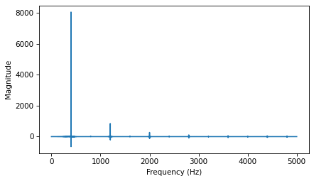
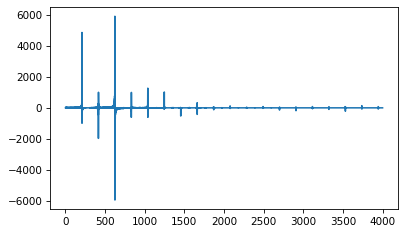
The result is the DCT of a triangle wave at 400 Hz, as shown in the following figure. The values of the DCT can be positive or negative; a negative value in the DCT corresponds to a negated cosine or, equivalently, to a cosine shifted by 180 degrees.

make_dct uses DCT-II, which is the most common type of DCT, provided by scipy.fftpack.

import scipy.fftpack

# class Wave:
def make_dct(self):
    N = len(self.ys)
    hs = scipy.fftpack.dct(self.ys, type=2)
    fs = (0.5 + np.arange(N)) / 2
    return Dct(hs, fs, self.framerate)

The results from dct are stored in hs. The corresponding frequencies, computed as in Section [dctiv]{reference-type=“ref” reference=“dctiv”}, are stored in fs. And then both are used to initialize the Dct object.

Dct provides make_wave, which performs the inverse DCT. We can test it like this:

wave2 = dct.make_wave()
max(abs(wave.ys-wave2.ys))
8.881784197001252e-16

The biggest difference between ys1 and ys2 is about 1e-16, which is what we expect due to floating-point errors.

make_wave uses scipy.fftpack.idct:

# class Dct
def make_wave(self):
    n = len(self.hs)
    ys = scipy.fftpack.idct(self.hs, type=2) / 2 / n
    return Wave(ys, framerate=self.framerate)

By default, the inverse DCT doesn’t normalize the result, so we have to divide through by \(2N\).

6.8. Exercises#

6.8.1. Exercise 6.1#

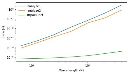
In this chapter I claim that analyze1 takes time proportional to \(n^3\) and analyze2 takes time proportional to \(n^2\). To see if that’s true, run them on a range of input sizes and time them. In IPython, you can use the magic command %timeit.

If you plot run time versus input size on a log-log scale, you should get a straight line with slope 3 for analyze1 and slope 2 for analyze2. You also might want to test dct_iv and scipy.fftpack.dct.

I’ll start with a noise signal and an array of power-of-two sizes

Hide code cell content

from thinkdsp import UncorrelatedGaussianNoise

signal = UncorrelatedGaussianNoise()
noise = signal.make_wave(duration=1.0, framerate=16384)
noise.ys.shape
(16384,)

The following function takes an array of results from a timing experiment, plots the results, and fits a straight line.

Hide code cell content

from scipy.stats import linregress

loglog = dict(xscale='log', yscale='log')

def plot_bests(ns, bests):    
    plt.plot(ns, bests)
    decorate(**loglog)
    
    x = np.log(ns)
    y = np.log(bests)
    t = linregress(x,y)
    slope = t[0]

    return slope

Hide code cell content

def analyze1(ys, fs, ts):
    """Analyze a mixture of cosines and return amplitudes.

    Works for the general case where M is not orthogonal.

    ys: wave array
    fs: frequencies in Hz
    ts: times where the signal was evaluated    
    
    returns: vector of amplitudes
    """
    args = np.outer(ts, fs)
    M = np.cos(PI2 * args)
    amps = np.linalg.solve(M, ys)
    return amps

Hide code cell content

def run_speed_test(ns, func):
    results = []
    for N in ns:
        print(N)
        ts = (0.5 + np.arange(N)) / N
        freqs = (0.5 + np.arange(N)) / 2
        ys = noise.ys[:N]
        result = %timeit -r1 -o func(ys, freqs, ts)
        results.append(result)
        
    bests = [result.best for result in results]
    return bests

Here are the results for analyze1.

Hide code cell content

ns = 2 ** np.arange(6, 13)
ns
array([  64,  128,  256,  512, 1024, 2048, 4096])

Hide code cell content

bests = run_speed_test(ns, analyze1)
plot_bests(ns, bests)
64
153 μs ± 0 ns per loop (mean ± std. dev. of 1 run, 10,000 loops each)
128
538 μs ± 0 ns per loop (mean ± std. dev. of 1 run, 1,000 loops each)
256
2.38 ms ± 0 ns per loop (mean ± std. dev. of 1 run, 100 loops each)
512
14.4 ms ± 0 ns per loop (mean ± std. dev. of 1 run, 100 loops each)
1024
73.5 ms ± 0 ns per loop (mean ± std. dev. of 1 run, 10 loops each)
2048
416 ms ± 0 ns per loop (mean ± std. dev. of 1 run, 1 loop each)
4096
2.93 s ± 0 ns per loop (mean ± std. dev. of 1 run, 1 loop each)
2.3866223708327747
_images/195439ac4ae80405c3a5c1443bcbb1f97d4bc65eeb4194cad312a81541ba277a.png

The estimated slope is close to 2, not 3, as expected. One possibility is that the performance of np.linalg.solve is nearly quadratic in this range of array sizes.

Here are the results for analyze2:

Hide code cell content

def analyze2(ys, fs, ts):
    """Analyze a mixture of cosines and return amplitudes.

    Assumes that fs and ts are chosen so that M is orthogonal.

    ys: wave array
    fs: frequencies in Hz
    ts: times where the signal was evaluated    
    
    returns: vector of amplitudes
    """
    args = np.outer(ts, fs)
    M = np.cos(PI2 * args)
    amps = np.dot(M, ys) / 2
    return amps

Hide code cell content

bests2 = run_speed_test(ns, analyze2)
plot_bests(ns, bests2)
64
89.4 μs ± 0 ns per loop (mean ± std. dev. of 1 run, 10,000 loops each)
128
339 μs ± 0 ns per loop (mean ± std. dev. of 1 run, 1,000 loops each)
256
1.42 ms ± 0 ns per loop (mean ± std. dev. of 1 run, 1,000 loops each)
512
5.19 ms ± 0 ns per loop (mean ± std. dev. of 1 run, 100 loops each)
1024
40.2 ms ± 0 ns per loop (mean ± std. dev. of 1 run, 10 loops each)
2048
129 ms ± 0 ns per loop (mean ± std. dev. of 1 run, 10 loops each)
4096
890 ms ± 0 ns per loop (mean ± std. dev. of 1 run, 1 loop each)
2.2077870325037
_images/0fc697c8d59b45b391141ba8262b77553d057b7fa68ff0583f47596596531504.png

The results for analyze2 fall in a straight line with the estimated slope close to 2, as expected.

Here are the results for the scipy.fftpack.dct

Hide code cell content

import scipy.fftpack

def scipy_dct(ys, freqs, ts):
    return scipy.fftpack.dct(ys, type=3)

Hide code cell content

bests3 = run_speed_test(ns, scipy_dct)
plot_bests(ns, bests3)
64
6.58 μs ± 0 ns per loop (mean ± std. dev. of 1 run, 100,000 loops each)
128
7.46 μs ± 0 ns per loop (mean ± std. dev. of 1 run, 100,000 loops each)
256
8.46 μs ± 0 ns per loop (mean ± std. dev. of 1 run, 100,000 loops each)
512
10.6 μs ± 0 ns per loop (mean ± std. dev. of 1 run, 100,000 loops each)
1024
14.5 μs ± 0 ns per loop (mean ± std. dev. of 1 run, 100,000 loops each)
2048
24.1 μs ± 0 ns per loop (mean ± std. dev. of 1 run, 10,000 loops each)
4096
41.3 μs ± 0 ns per loop (mean ± std. dev. of 1 run, 10,000 loops each)
0.43247225316739907
_images/b95333c8a3bf8e8fd17a0098fd97478ba7078ff7bbeb572f0812cb4c677c5c49.png

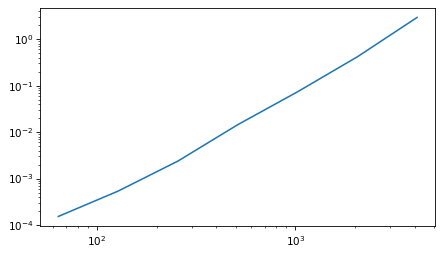
This implementation of dct is even faster. The line is curved, which means either we haven’t seen the asymptotic behavior yet, or the asymptotic behavior is not a simple exponent of \(n\). In fact, as we’ll see soon, the run time is proportional to \(n \log n\).

The following figure shows all three curves on the same axes.

Hide code cell content

plt.plot(ns, bests, label='analyze1')
plt.plot(ns, bests2, label='analyze2')
plt.plot(ns, bests3, label='fftpack.dct')
decorate(xlabel='Wave length (N)', ylabel='Time (s)', **loglog)
_images/efb192a3bfc501fdeea3b9663b60e394d2d9dbb5566eca3310f296f457f8e377.png

6.8.2. Exercise 6.2#

One of the major applications of the DCT is compression for both sound and images. In its simplest form, DCT-based compression works like this:

  1. Break a long signal into segments.

  2. Compute the DCT of each segment.

  3. Identify frequency components with amplitudes so low they are inaudible, and remove them. Store only the frequencies and amplitudes that remain.

  4. To play back the signal, load the frequencies and amplitudes for each segment and apply the inverse DCT.

Implement a version of this algorithm and apply it to a recording of music or speech. How many components can you eliminate before the difference is perceptible?

thinkdsp provides a class, Dct that is similar to a Spectrum, but which uses DCT instead of FFT.

As an example, I’ll use a recording of a saxophone:

Hide code cell content

download('https://github.com/AllenDowney/ThinkDSP/raw/master/code/100475__iluppai__saxophone-weep.wav')

Hide code cell content

from thinkdsp import read_wave

wave = read_wave('100475__iluppai__saxophone-weep.wav')
wave.make_audio()

Here’s a short segment:

Hide code cell content

segment = wave.segment(start=1.2, duration=0.5)
segment.normalize()
segment.make_audio()

And here’s the DCT of that segment:

Hide code cell content

seg_dct = segment.make_dct()
seg_dct.plot(high=4000)
decorate_freq()
_images/815ebd398cbe7ca22f9b43d37ab6195f12c90ba1826bfe1d8dc577e5dcb2a8e1.png

There are only a few harmonics with substantial amplitude, and many entries near zero.

The following function takes a DCT and sets elements below thresh to 0.

Hide code cell content

def compress(dct, thresh=1):
    count = 0
    for i, amp in enumerate(dct.amps):
        if np.abs(amp) < thresh:
            dct.hs[i] = 0
            count += 1
            
    n = len(dct.amps)
    print(count, n, 100 * count / n, sep='\t')

If we apply it to the segment, we can eliminate more than 90% of the elements:

Hide code cell content

seg_dct = segment.make_dct()
compress(seg_dct, thresh=10)
seg_dct.plot(high=4000)
20457	22050	92.77551020408163
_images/79ecee41011a06eb9be178fd411028762d809a2042677fcdaedb3bab8ae1c547.png

And the result sounds the same (at least to me):

Hide code cell content

seg2 = seg_dct.make_wave()
seg2.make_audio()

To compress a longer segment, we can make a DCT spectrogram. The following function is similar to wave.make_spectrogram except that it uses the DCT.

Hide code cell content

from thinkdsp import Spectrogram

def make_dct_spectrogram(wave, seg_length):
    """Computes the DCT spectrogram of the wave.

    seg_length: number of samples in each segment

    returns: Spectrogram
    """
    window = np.hamming(seg_length)
    i, j = 0, seg_length
    step = seg_length // 2

    # map from time to Spectrum
    spec_map = {}

    while j < len(wave.ys):
        segment = wave.slice(i, j)
        segment.window(window)

        # the nominal time for this segment is the midpoint
        t = (segment.start + segment.end) / 2
        spec_map[t] = segment.make_dct()

        i += step
        j += step

    return Spectrogram(spec_map, seg_length)

Now we can make a DCT spectrogram and apply compress to each segment:

Hide code cell content

spectro = make_dct_spectrogram(wave, seg_length=1024)
for t, dct in sorted(spectro.spec_map.items()):
    compress(dct, thresh=0.2)
1018	1024	99.4140625
1016	1024	99.21875
1014	1024	99.0234375
1017	1024	99.31640625
1016	1024	99.21875
1017	1024	99.31640625
1016	1024	99.21875
1020	1024	99.609375
1014	1024	99.0234375
1005	1024	98.14453125
1009	1024	98.53515625
1015	1024	99.12109375
1015	1024	99.12109375
1016	1024	99.21875
1016	1024	99.21875
1015	1024	99.12109375
1017	1024	99.31640625
1020	1024	99.609375
1013	1024	98.92578125
1017	1024	99.31640625
1013	1024	98.92578125
1017	1024	99.31640625
1018	1024	99.4140625
1015	1024	99.12109375
1013	1024	98.92578125
794	1024	77.5390625
785	1024	76.66015625
955	1024	93.26171875
995	1024	97.16796875
992	1024	96.875
976	1024	95.3125
925	1024	90.33203125
802	1024	78.3203125
836	1024	81.640625
850	1024	83.0078125
882	1024	86.1328125
883	1024	86.23046875
891	1024	87.01171875
901	1024	87.98828125
902	1024	88.0859375
900	1024	87.890625
900	1024	87.890625
894	1024	87.3046875
904	1024	88.28125
901	1024	87.98828125
915	1024	89.35546875
913	1024	89.16015625
899	1024	87.79296875
905	1024	88.37890625
905	1024	88.37890625
888	1024	86.71875
898	1024	87.6953125
879	1024	85.83984375
893	1024	87.20703125
893	1024	87.20703125
882	1024	86.1328125
874	1024	85.3515625
876	1024	85.546875
864	1024	84.375
879	1024	85.83984375
869	1024	84.86328125
872	1024	85.15625
871	1024	85.05859375
878	1024	85.7421875
872	1024	85.15625
859	1024	83.88671875
879	1024	85.83984375
889	1024	86.81640625
872	1024	85.15625
837	1024	81.73828125
842	1024	82.2265625
825	1024	80.56640625
839	1024	81.93359375
796	1024	77.734375
792	1024	77.34375
769	1024	75.09765625
836	1024	81.640625
919	1024	89.74609375
913	1024	89.16015625
942	1024	91.9921875
837	1024	81.73828125
739	1024	72.16796875
737	1024	71.97265625
726	1024	70.8984375
728	1024	71.09375
733	1024	71.58203125
717	1024	70.01953125
716	1024	69.921875
676	1024	66.015625
712	1024	69.53125
697	1024	68.06640625
718	1024	70.1171875
717	1024	70.01953125
718	1024	70.1171875
681	1024	66.50390625
707	1024	69.04296875
691	1024	67.48046875
681	1024	66.50390625
709	1024	69.23828125
684	1024	66.796875
743	1024	72.55859375
710	1024	69.3359375
712	1024	69.53125
714	1024	69.7265625
719	1024	70.21484375
708	1024	69.140625
725	1024	70.80078125
700	1024	68.359375
726	1024	70.8984375
716	1024	69.921875
725	1024	70.80078125
692	1024	67.578125
675	1024	65.91796875
747	1024	72.94921875
741	1024	72.36328125
730	1024	71.2890625
701	1024	68.45703125
721	1024	70.41015625
747	1024	72.94921875
725	1024	70.80078125
744	1024	72.65625
720	1024	70.3125
716	1024	69.921875
723	1024	70.60546875
721	1024	70.41015625
734	1024	71.6796875
730	1024	71.2890625
718	1024	70.1171875
730	1024	71.2890625
723	1024	70.60546875
749	1024	73.14453125
727	1024	70.99609375
728	1024	71.09375
746	1024	72.8515625
739	1024	72.16796875
757	1024	73.92578125
741	1024	72.36328125
751	1024	73.33984375
775	1024	75.68359375
749	1024	73.14453125
768	1024	75.0
763	1024	74.51171875
771	1024	75.29296875
758	1024	74.0234375
745	1024	72.75390625
756	1024	73.828125
744	1024	72.65625
743	1024	72.55859375
757	1024	73.92578125
779	1024	76.07421875
760	1024	74.21875
770	1024	75.1953125
759	1024	74.12109375
737	1024	71.97265625
739	1024	72.16796875
751	1024	73.33984375
762	1024	74.4140625
754	1024	73.6328125
811	1024	79.19921875
899	1024	87.79296875
832	1024	81.25
800	1024	78.125
756	1024	73.828125
748	1024	73.046875
727	1024	70.99609375
744	1024	72.65625
725	1024	70.80078125
720	1024	70.3125
755	1024	73.73046875
737	1024	71.97265625
766	1024	74.8046875
747	1024	72.94921875
743	1024	72.55859375
727	1024	70.99609375
726	1024	70.8984375
746	1024	72.8515625
764	1024	74.609375
751	1024	73.33984375
734	1024	71.6796875
741	1024	72.36328125
760	1024	74.21875
750	1024	73.2421875
784	1024	76.5625
730	1024	71.2890625
757	1024	73.92578125
761	1024	74.31640625
734	1024	71.6796875
744	1024	72.65625
757	1024	73.92578125
714	1024	69.7265625
740	1024	72.265625
738	1024	72.0703125
763	1024	74.51171875
766	1024	74.8046875
745	1024	72.75390625
751	1024	73.33984375
759	1024	74.12109375
756	1024	73.828125
756	1024	73.828125
756	1024	73.828125
755	1024	73.73046875
746	1024	72.8515625
756	1024	73.828125
738	1024	72.0703125
757	1024	73.92578125
764	1024	74.609375
765	1024	74.70703125
762	1024	74.4140625
768	1024	75.0
773	1024	75.48828125
782	1024	76.3671875
773	1024	75.48828125
766	1024	74.8046875
755	1024	73.73046875
766	1024	74.8046875
772	1024	75.390625
810	1024	79.1015625
739	1024	72.16796875
717	1024	70.01953125
722	1024	70.5078125
739	1024	72.16796875
725	1024	70.80078125
736	1024	71.875
759	1024	74.12109375
769	1024	75.09765625
749	1024	73.14453125
710	1024	69.3359375
748	1024	73.046875
720	1024	70.3125
732	1024	71.484375
721	1024	70.41015625
734	1024	71.6796875
763	1024	74.51171875
747	1024	72.94921875
754	1024	73.6328125
755	1024	73.73046875
764	1024	74.609375
801	1024	78.22265625
768	1024	75.0
780	1024	76.171875
773	1024	75.48828125
764	1024	74.609375
775	1024	75.68359375
740	1024	72.265625
794	1024	77.5390625
796	1024	77.734375
769	1024	75.09765625
751	1024	73.33984375
782	1024	76.3671875
758	1024	74.0234375
777	1024	75.87890625
794	1024	77.5390625
784	1024	76.5625
788	1024	76.953125
773	1024	75.48828125
783	1024	76.46484375
784	1024	76.5625
785	1024	76.66015625
806	1024	78.7109375
807	1024	78.80859375
797	1024	77.83203125
785	1024	76.66015625
794	1024	77.5390625
766	1024	74.8046875
790	1024	77.1484375
746	1024	72.8515625
762	1024	74.4140625
813	1024	79.39453125
801	1024	78.22265625
782	1024	76.3671875
776	1024	75.78125
755	1024	73.73046875
780	1024	76.171875
784	1024	76.5625
805	1024	78.61328125
791	1024	77.24609375
803	1024	78.41796875
799	1024	78.02734375
795	1024	77.63671875
797	1024	77.83203125
806	1024	78.7109375
781	1024	76.26953125
795	1024	77.63671875
797	1024	77.83203125
893	1024	87.20703125
775	1024	75.68359375
787	1024	76.85546875
746	1024	72.8515625
767	1024	74.90234375
749	1024	73.14453125
749	1024	73.14453125
738	1024	72.0703125
736	1024	71.875
747	1024	72.94921875
760	1024	74.21875
737	1024	71.97265625
752	1024	73.4375
756	1024	73.828125
772	1024	75.390625
740	1024	72.265625
737	1024	71.97265625
766	1024	74.8046875
791	1024	77.24609375
765	1024	74.70703125
771	1024	75.29296875
786	1024	76.7578125
770	1024	75.1953125
761	1024	74.31640625
765	1024	74.70703125
756	1024	73.828125
758	1024	74.0234375
765	1024	74.70703125
785	1024	76.66015625
769	1024	75.09765625
781	1024	76.26953125
792	1024	77.34375
798	1024	77.9296875
809	1024	79.00390625
778	1024	75.9765625
782	1024	76.3671875
776	1024	75.78125
791	1024	77.24609375
794	1024	77.5390625
783	1024	76.46484375
771	1024	75.29296875
792	1024	77.34375
785	1024	76.66015625
812	1024	79.296875
809	1024	79.00390625
799	1024	78.02734375
798	1024	77.9296875
803	1024	78.41796875
800	1024	78.125
805	1024	78.61328125
803	1024	78.41796875
799	1024	78.02734375
802	1024	78.3203125
804	1024	78.515625
809	1024	79.00390625
784	1024	76.5625
791	1024	77.24609375
814	1024	79.4921875
788	1024	76.953125
816	1024	79.6875
810	1024	79.1015625
820	1024	80.078125
823	1024	80.37109375
813	1024	79.39453125
799	1024	78.02734375
807	1024	78.80859375
799	1024	78.02734375
789	1024	77.05078125
813	1024	79.39453125
819	1024	79.98046875
809	1024	79.00390625
784	1024	76.5625
809	1024	79.00390625
810	1024	79.1015625
785	1024	76.66015625
838	1024	81.8359375
821	1024	80.17578125
822	1024	80.2734375
800	1024	78.125
815	1024	79.58984375
827	1024	80.76171875
820	1024	80.078125
792	1024	77.34375
818	1024	79.8828125
813	1024	79.39453125
824	1024	80.46875
795	1024	77.63671875
788	1024	76.953125
796	1024	77.734375
802	1024	78.3203125
800	1024	78.125
796	1024	77.734375
823	1024	80.37109375
804	1024	78.515625
811	1024	79.19921875
808	1024	78.90625
815	1024	79.58984375
812	1024	79.296875
822	1024	80.2734375
793	1024	77.44140625
803	1024	78.41796875
806	1024	78.7109375
812	1024	79.296875
796	1024	77.734375
804	1024	78.515625
807	1024	78.80859375
821	1024	80.17578125
793	1024	77.44140625
799	1024	78.02734375
810	1024	79.1015625
818	1024	79.8828125
813	1024	79.39453125
825	1024	80.56640625
804	1024	78.515625
821	1024	80.17578125
809	1024	79.00390625
828	1024	80.859375
813	1024	79.39453125
838	1024	81.8359375
836	1024	81.640625
818	1024	79.8828125
808	1024	78.90625
819	1024	79.98046875
820	1024	80.078125
814	1024	79.4921875
901	1024	87.98828125
894	1024	87.3046875
888	1024	86.71875
780	1024	76.171875
773	1024	75.48828125
750	1024	73.2421875
750	1024	73.2421875
730	1024	71.2890625
761	1024	74.31640625
775	1024	75.68359375
782	1024	76.3671875
788	1024	76.953125
748	1024	73.046875
752	1024	73.4375
771	1024	75.29296875
746	1024	72.8515625
778	1024	75.9765625
777	1024	75.87890625
760	1024	74.21875
734	1024	71.6796875
711	1024	69.43359375
754	1024	73.6328125
745	1024	72.75390625
758	1024	74.0234375
744	1024	72.65625
755	1024	73.73046875
749	1024	73.14453125
723	1024	70.60546875
784	1024	76.5625
761	1024	74.31640625
758	1024	74.0234375
709	1024	69.23828125
769	1024	75.09765625
773	1024	75.48828125
769	1024	75.09765625
756	1024	73.828125
747	1024	72.94921875
787	1024	76.85546875
770	1024	75.1953125
749	1024	73.14453125
769	1024	75.09765625
748	1024	73.046875
761	1024	74.31640625
759	1024	74.12109375
775	1024	75.68359375
756	1024	73.828125
774	1024	75.5859375
776	1024	75.78125
760	1024	74.21875
783	1024	76.46484375
744	1024	72.65625
766	1024	74.8046875
761	1024	74.31640625
788	1024	76.953125
774	1024	75.5859375
753	1024	73.53515625
754	1024	73.6328125
765	1024	74.70703125
736	1024	71.875
782	1024	76.3671875
768	1024	75.0
778	1024	75.9765625
767	1024	74.90234375
774	1024	75.5859375
772	1024	75.390625
769	1024	75.09765625
774	1024	75.5859375
776	1024	75.78125
796	1024	77.734375
762	1024	74.4140625
766	1024	74.8046875
765	1024	74.70703125
783	1024	76.46484375
770	1024	75.1953125
799	1024	78.02734375
779	1024	76.07421875
774	1024	75.5859375
791	1024	77.24609375
797	1024	77.83203125
781	1024	76.26953125
754	1024	73.6328125
790	1024	77.1484375
790	1024	77.1484375
801	1024	78.22265625
783	1024	76.46484375
787	1024	76.85546875
805	1024	78.61328125
758	1024	74.0234375
785	1024	76.66015625
788	1024	76.953125
806	1024	78.7109375
818	1024	79.8828125
776	1024	75.78125
807	1024	78.80859375
802	1024	78.3203125
782	1024	76.3671875
812	1024	79.296875
803	1024	78.41796875
803	1024	78.41796875
787	1024	76.85546875
799	1024	78.02734375
786	1024	76.7578125
813	1024	79.39453125
813	1024	79.39453125
813	1024	79.39453125
803	1024	78.41796875
815	1024	79.58984375
792	1024	77.34375
807	1024	78.80859375
829	1024	80.95703125
797	1024	77.83203125
814	1024	79.4921875
793	1024	77.44140625
802	1024	78.3203125
775	1024	75.68359375
816	1024	79.6875
804	1024	78.515625
808	1024	78.90625
809	1024	79.00390625
814	1024	79.4921875
808	1024	78.90625
823	1024	80.37109375
811	1024	79.19921875
806	1024	78.7109375
819	1024	79.98046875
805	1024	78.61328125
826	1024	80.6640625
826	1024	80.6640625
807	1024	78.80859375
818	1024	79.8828125
818	1024	79.8828125
812	1024	79.296875
816	1024	79.6875
815	1024	79.58984375
827	1024	80.76171875
830	1024	81.0546875
852	1024	83.203125
827	1024	80.76171875
834	1024	81.4453125
835	1024	81.54296875
835	1024	81.54296875
829	1024	80.95703125
822	1024	80.2734375
818	1024	79.8828125
827	1024	80.76171875
834	1024	81.4453125
829	1024	80.95703125
846	1024	82.6171875
829	1024	80.95703125
829	1024	80.95703125
833	1024	81.34765625
837	1024	81.73828125
837	1024	81.73828125
815	1024	79.58984375
834	1024	81.4453125
833	1024	81.34765625
840	1024	82.03125
855	1024	83.49609375
853	1024	83.30078125
853	1024	83.30078125
846	1024	82.6171875
852	1024	83.203125
856	1024	83.59375
859	1024	83.88671875
851	1024	83.10546875
845	1024	82.51953125
874	1024	85.3515625
861	1024	84.08203125
877	1024	85.64453125
853	1024	83.30078125
861	1024	84.08203125
859	1024	83.88671875
866	1024	84.5703125
868	1024	84.765625
870	1024	84.9609375
856	1024	83.59375
859	1024	83.88671875
864	1024	84.375
864	1024	84.375
876	1024	85.546875
872	1024	85.15625
872	1024	85.15625
863	1024	84.27734375
859	1024	83.88671875
878	1024	85.7421875
860	1024	83.984375
864	1024	84.375
875	1024	85.44921875
862	1024	84.1796875
867	1024	84.66796875
867	1024	84.66796875
864	1024	84.375
864	1024	84.375
876	1024	85.546875
875	1024	85.44921875
860	1024	83.984375
865	1024	84.47265625
881	1024	86.03515625
867	1024	84.66796875
869	1024	84.86328125
873	1024	85.25390625
869	1024	84.86328125
873	1024	85.25390625
873	1024	85.25390625
862	1024	84.1796875
865	1024	84.47265625
871	1024	85.05859375
869	1024	84.86328125
871	1024	85.05859375
866	1024	84.5703125
877	1024	85.64453125
861	1024	84.08203125
881	1024	86.03515625
882	1024	86.1328125
874	1024	85.3515625
875	1024	85.44921875
866	1024	84.5703125
870	1024	84.9609375
883	1024	86.23046875
870	1024	84.9609375
871	1024	85.05859375
877	1024	85.64453125
866	1024	84.5703125
877	1024	85.64453125
863	1024	84.27734375
873	1024	85.25390625
871	1024	85.05859375
883	1024	86.23046875
862	1024	84.1796875
853	1024	83.30078125
858	1024	83.7890625
857	1024	83.69140625
855	1024	83.49609375
847	1024	82.71484375
837	1024	81.73828125
850	1024	83.0078125
864	1024	84.375
879	1024	85.83984375
883	1024	86.23046875
871	1024	85.05859375
888	1024	86.71875
881	1024	86.03515625
830	1024	81.0546875
870	1024	84.9609375
877	1024	85.64453125
886	1024	86.5234375
863	1024	84.27734375
871	1024	85.05859375
886	1024	86.5234375
871	1024	85.05859375
896	1024	87.5
872	1024	85.15625
870	1024	84.9609375
877	1024	85.64453125
863	1024	84.27734375
886	1024	86.5234375
898	1024	87.6953125
884	1024	86.328125
908	1024	88.671875
878	1024	85.7421875
865	1024	84.47265625
864	1024	84.375
888	1024	86.71875
870	1024	84.9609375
862	1024	84.1796875
866	1024	84.5703125
889	1024	86.81640625
879	1024	85.83984375
884	1024	86.328125
880	1024	85.9375
876	1024	85.546875
864	1024	84.375
877	1024	85.64453125
858	1024	83.7890625
894	1024	87.3046875
890	1024	86.9140625
893	1024	87.20703125
891	1024	87.01171875
896	1024	87.5
892	1024	87.109375
906	1024	88.4765625
878	1024	85.7421875
893	1024	87.20703125
898	1024	87.6953125
888	1024	86.71875
903	1024	88.18359375
911	1024	88.96484375
911	1024	88.96484375
901	1024	87.98828125
909	1024	88.76953125
911	1024	88.96484375
921	1024	89.94140625
922	1024	90.0390625
916	1024	89.453125
923	1024	90.13671875
928	1024	90.625
920	1024	89.84375
922	1024	90.0390625
915	1024	89.35546875
930	1024	90.8203125
914	1024	89.2578125
917	1024	89.55078125
918	1024	89.6484375
921	1024	89.94140625
921	1024	89.94140625
937	1024	91.50390625
931	1024	90.91796875
923	1024	90.13671875
921	1024	89.94140625
934	1024	91.2109375
930	1024	90.8203125
933	1024	91.11328125
932	1024	91.015625
930	1024	90.8203125
930	1024	90.8203125
933	1024	91.11328125
933	1024	91.11328125
949	1024	92.67578125
941	1024	91.89453125
945	1024	92.28515625
936	1024	91.40625
956	1024	93.359375
948	1024	92.578125
936	1024	91.40625
941	1024	91.89453125
949	1024	92.67578125
941	1024	91.89453125
940	1024	91.796875
951	1024	92.87109375
941	1024	91.89453125
941	1024	91.89453125
930	1024	90.8203125
930	1024	90.8203125
924	1024	90.234375
919	1024	89.74609375
911	1024	88.96484375
934	1024	91.2109375
892	1024	87.109375
929	1024	90.72265625
922	1024	90.0390625
927	1024	90.52734375
917	1024	89.55078125
856	1024	83.59375
835	1024	81.54296875
852	1024	83.203125
870	1024	84.9609375
878	1024	85.7421875
872	1024	85.15625
894	1024	87.3046875
865	1024	84.47265625
889	1024	86.81640625
871	1024	85.05859375
873	1024	85.25390625
864	1024	84.375
859	1024	83.88671875
867	1024	84.66796875
833	1024	81.34765625
853	1024	83.30078125
874	1024	85.3515625
843	1024	82.32421875
848	1024	82.8125
844	1024	82.421875
817	1024	79.78515625
865	1024	84.47265625
807	1024	78.80859375
752	1024	73.4375
775	1024	75.68359375
772	1024	75.390625
778	1024	75.9765625
767	1024	74.90234375
784	1024	76.5625
800	1024	78.125
807	1024	78.80859375
826	1024	80.6640625
805	1024	78.61328125
788	1024	76.953125
820	1024	80.078125
809	1024	79.00390625
803	1024	78.41796875
799	1024	78.02734375
806	1024	78.7109375
839	1024	81.93359375
846	1024	82.6171875
914	1024	89.2578125
888	1024	86.71875
839	1024	81.93359375
836	1024	81.640625
830	1024	81.0546875
845	1024	82.51953125
828	1024	80.859375
834	1024	81.4453125
854	1024	83.3984375
847	1024	82.71484375
846	1024	82.6171875
845	1024	82.51953125
863	1024	84.27734375
867	1024	84.66796875
855	1024	83.49609375
844	1024	82.421875
864	1024	84.375
865	1024	84.47265625
860	1024	83.984375
868	1024	84.765625
871	1024	85.05859375
868	1024	84.765625
857	1024	83.69140625
885	1024	86.42578125
908	1024	88.671875
872	1024	85.15625
848	1024	82.8125
813	1024	79.39453125
763	1024	74.51171875
761	1024	74.31640625
779	1024	76.07421875
783	1024	76.46484375
776	1024	75.78125
784	1024	76.5625
811	1024	79.19921875
812	1024	79.296875
777	1024	75.87890625
794	1024	77.5390625
794	1024	77.5390625
813	1024	79.39453125
805	1024	78.61328125
828	1024	80.859375
796	1024	77.734375
806	1024	78.7109375
817	1024	79.78515625
840	1024	82.03125
786	1024	76.7578125
818	1024	79.8828125
832	1024	81.25
835	1024	81.54296875
768	1024	75.0
841	1024	82.12890625
833	1024	81.34765625
836	1024	81.640625
824	1024	80.46875
830	1024	81.0546875
837	1024	81.73828125
837	1024	81.73828125
858	1024	83.7890625
847	1024	82.71484375
870	1024	84.9609375
866	1024	84.5703125
843	1024	82.32421875
867	1024	84.66796875
849	1024	82.91015625
869	1024	84.86328125
860	1024	83.984375
862	1024	84.1796875
846	1024	82.6171875
854	1024	83.3984375
871	1024	85.05859375
861	1024	84.08203125
882	1024	86.1328125
892	1024	87.109375
877	1024	85.64453125
895	1024	87.40234375
887	1024	86.62109375
873	1024	85.25390625
894	1024	87.3046875
890	1024	86.9140625
878	1024	85.7421875
894	1024	87.3046875
879	1024	85.83984375
890	1024	86.9140625
895	1024	87.40234375
889	1024	86.81640625
896	1024	87.5
898	1024	87.6953125
901	1024	87.98828125
879	1024	85.83984375
890	1024	86.9140625
888	1024	86.71875
917	1024	89.55078125
902	1024	88.0859375
921	1024	89.94140625
915	1024	89.35546875
927	1024	90.52734375
923	1024	90.13671875
928	1024	90.625
923	1024	90.13671875
914	1024	89.2578125
918	1024	89.6484375
927	1024	90.52734375
926	1024	90.4296875
919	1024	89.74609375
916	1024	89.453125
928	1024	90.625
916	1024	89.453125
933	1024	91.11328125
925	1024	90.33203125
930	1024	90.8203125
930	1024	90.8203125
934	1024	91.2109375
933	1024	91.11328125
935	1024	91.30859375
939	1024	91.69921875
934	1024	91.2109375
938	1024	91.6015625
944	1024	92.1875
937	1024	91.50390625
937	1024	91.50390625
935	1024	91.30859375
937	1024	91.50390625
937	1024	91.50390625
954	1024	93.1640625
940	1024	91.796875
942	1024	91.9921875
955	1024	93.26171875
949	1024	92.67578125
941	1024	91.89453125
947	1024	92.48046875
940	1024	91.796875
943	1024	92.08984375
946	1024	92.3828125
962	1024	93.9453125
954	1024	93.1640625
956	1024	93.359375
957	1024	93.45703125
962	1024	93.9453125
960	1024	93.75
944	1024	92.1875
969	1024	94.62890625
969	1024	94.62890625
969	1024	94.62890625
968	1024	94.53125
970	1024	94.7265625
969	1024	94.62890625
975	1024	95.21484375
963	1024	94.04296875
965	1024	94.23828125
975	1024	95.21484375
969	1024	94.62890625
966	1024	94.3359375
969	1024	94.62890625
984	1024	96.09375
981	1024	95.80078125
977	1024	95.41015625
982	1024	95.8984375
980	1024	95.703125
980	1024	95.703125
981	1024	95.80078125
982	1024	95.8984375
981	1024	95.80078125
987	1024	96.38671875
982	1024	95.8984375
982	1024	95.8984375
977	1024	95.41015625
982	1024	95.8984375
986	1024	96.2890625
984	1024	96.09375
986	1024	96.2890625
987	1024	96.38671875
996	1024	97.265625
995	1024	97.16796875
997	1024	97.36328125
999	1024	97.55859375
1002	1024	97.8515625
999	1024	97.55859375
1004	1024	98.046875
1002	1024	97.8515625
999	1024	97.55859375
1000	1024	97.65625
1007	1024	98.33984375
1010	1024	98.6328125
1012	1024	98.828125
1004	1024	98.046875
1000	1024	97.65625
1008	1024	98.4375
1005	1024	98.14453125
1011	1024	98.73046875
1011	1024	98.73046875
1009	1024	98.53515625
1005	1024	98.14453125
1007	1024	98.33984375
1010	1024	98.6328125
1010	1024	98.6328125
1005	1024	98.14453125
1008	1024	98.4375
1012	1024	98.828125
1009	1024	98.53515625
1012	1024	98.828125
1013	1024	98.92578125
1010	1024	98.6328125
1012	1024	98.828125
1014	1024	99.0234375
1016	1024	99.21875
1010	1024	98.6328125
1014	1024	99.0234375
1015	1024	99.12109375
1012	1024	98.828125
1019	1024	99.51171875
1015	1024	99.12109375
1016	1024	99.21875
1019	1024	99.51171875
1019	1024	99.51171875
1016	1024	99.21875
1018	1024	99.4140625
1018	1024	99.4140625

In most segments, the compression is 75-85%.

To hear what it sounds like, we can convert the spectrogram back to a wave and play it.

Hide code cell content

wave2 = spectro.make_wave()
wave2.make_audio()

And here’s the original again for comparison.

Hide code cell content

wave.make_audio()

As an experiment, you might try increasing thresh to see when the effect of compression becomes audible (to you).

Also, you might try compressing a signal with some noisy elements, like cymbals.

Think DSP: Digital Signal Processing in Python, 2nd Edition

Copyright 2024 Allen B. Downey

License: Creative Commons Attribution-NonCommercial-ShareAlike 4.0 International