This is Part 5 in a series on gender gaps in life expectancy, what causes them, and what we can do about it.
The HALE Gap
So far we’ve focused on life expectancy, but the Global Gender Gap Report (GGGR) we cited in Part 1 uses healthy life expectancy (HALE), which is expected years of good health. So we’ll repeat the analysis we did with life expectancy, this time with HALE data from the IHME Global Burden of Disease.
The following figure shows the gender gap in HALE (female minus male) for OECD countries from 2000 to 2023.
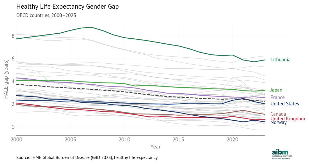
HALE gender gap (2000–2023), OECD countries.
In 2023, the average HALE gap was 2.2 years, smaller than the average life expectancy gap, which was 5.1 years. This difference suggests that some of the additional years that women live are not spent in good health.
The trends in HALE are similar to the trends in life expectancy: decreasing in most countries, except during the COVID pandemic -- and increasing in the United States and Canada, primarily due to the opioid epidemic.
The 2025 GGGR notes these decreasing gaps and concludes:
While overall life expectancy by gender has remained more stable than healthy life expectancy, and women continue to outlive men, this indicates that the proportion of women’s lives spent in full health has declined relative to men.
This interpretation makes it sound like women’s health outcomes are getting worse, but they are not. The following figure shows HALE over time for OECD countries, with green lines for men and purple for women. As examples, it highlights the countries with the largest and smallest gaps, Lithuania and Norway.
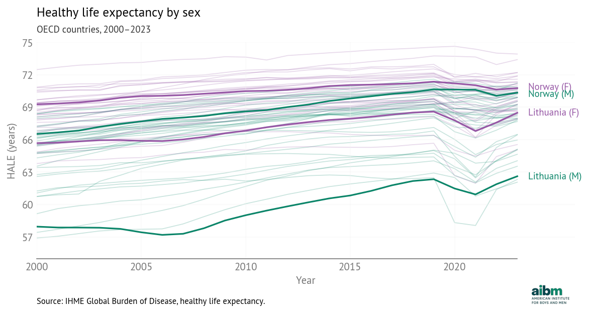
Healthy life expectancy by sex, OECD 2000–2023 (IHME).
The HALE gap is narrowing in 34 out of 37 countries -- and in every one of them HALE is increasing for both men and women. Because men generally suffer worse health outcomes, as health outcomes improve, they improve faster for men, closing the gap.
To look at these trends and say, as WEF did, that women’s health has “declined relative to men” is strange and misleading.
The Model
With the HALE data, we ran a Bayesian hierarchical model with the same predictors as the life expectancy model in Part 2. The following figure shows the estimated coefficients.
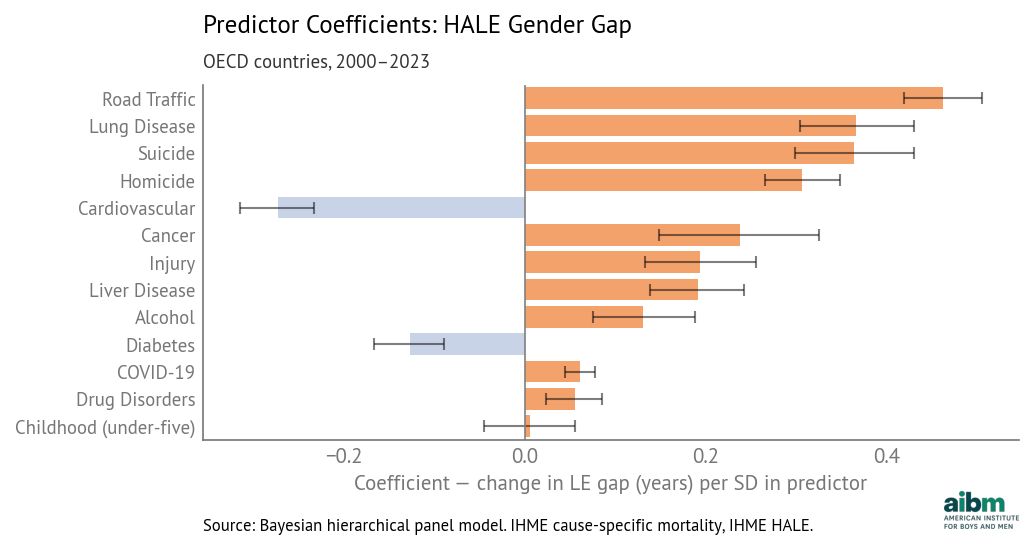
Predictor coefficients for the HALE gender gap (posterior mean and 94% intervals). OECD, 2000–2023.
Road traffic deaths have the largest coefficient, about 0.46 years per standard deviation, which means that if a country is average except that its traffic death gap is one standard deviation above the mean, we expect its HALE gap to be 0.46 years above average. Other factors with large coefficients are lung disease, suicide, and homicide.
The coefficients for cardiovascular disease and diabetes are negative, as in the life expectancy model. As we discussed in Part 2, a likely explanation is competing risks -- where rates are lower for causes that affect young people, rates are higher for diseases of aging.
The following table shows the coefficient for each cause, sorted by magnitude, and the rank of each cause in the two models.
| Cause | Coefficient | Rank (HALE) | Rank (LE) |
|---|---|---|---|
| Road traffic | 0.463 | 1 | 1 |
| Lung disease | 0.367 | 2 | 5 |
| Suicide | 0.364 | 3 | 3 |
| Homicide | 0.307 | 4 | 2 |
| Cardiovascular | −0.273 | 5 | 7 |
| Cancer | 0.238 | 6 | 4 |
| Unintentional injury | 0.194 | 7 | 8 |
| Liver disease | 0.191 | 8 | 6 |
| Alcohol | 0.130 | 9 | 9 |
| Diabetes | −0.128 | 10 | 12 |
| COVID-19 | 0.060 | 11 | 10 |
| Drug disorders | 0.055 | 12 | 11 |
| Childhood (under-five) | 0.005 | 13 | 13 |
The rankings are consistent. The biggest difference is that lung disease, which has the fifth largest coefficient in the life expectancy model, moves up to second in the HALE model. The other differences are small and within expected variability.
For each cause of death, we also computed “importances”, as explained in Part 2. The results are consistent -- comparing the rankings from the HALE and life expectancy models, each cause of death appears higher or lower in the list by at most two spots.
Goodness of fit
The model fits the data well. The following figure shows the residuals (actual gaps minus the predictions from the model) for each country.
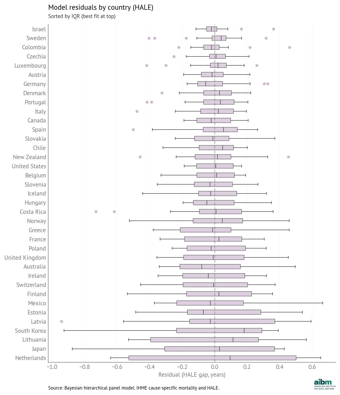
HALE model residuals by country (years); same layout as LE.
Most errors are less than 0.5 years and all are less than 1.0 years. The predictions are mostly unbiased -- that is, the average error for most countries is close to zero.
Counterfactuals
Using the method described in Part 3 we predicted counterfactual HALE for each country, assuming that each death-rate gap could be lowered to the best observed value.
The following table shows the results for the United States in 2023.
| Cause | Current gap | Target gap | Target Country-Year | Change in HALE gap (years) |
|---|---|---|---|---|
| Road Traffic | 13 | 1.92 | Iceland (2017) | -0.86 |
| Suicide | 17.7 | 4.05 | Greece (2002) | -0.52 |
| Drug Disorders | 23.6 | 0.0028 | Japan (2013) | -0.47 |
| Homicide | 8.85 | 0 | -0.20 | |
| Liver Disease | 9.06 | 0.729 | Iceland (2001) | -0.16 |
| Alcohol | 7.37 | 0.232 | Colombia (2016) | -0.15 |
| Cancer | 23.5 | 0 | -0.15 | |
| Injury | 5.9 | 0 | -0.08 | |
| COVID-19 | 1.28 | 0 | -0.01 | |
| Childhood (under-five) | 23.2 | 0.594 | Ireland (2021) | -0.01 |
| Lung Disease | -6.32 | 0 | 0.22 | |
| Cardiovascular | 30.7 | 0 | 0.23 | |
| Diabetes | 7.73 | 0 | 0.28 |
This figure shows the counterfactual effects graphically.
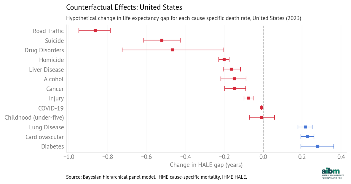
HALE: hypothetical change in predicted gap, USA 2023, with 94% credible intervals.
The leading contributors in the HALE model are the same as in the life expectancy model. The top factor is road traffic -- if the death-rate gap could be reduced from 13 to 1.92 per 100,000, the model predicts that the HALE gap would be reduced by 0.86 years.
The following figure shows how these contributions have changed over time.
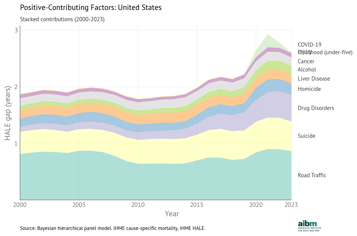
HALE: stacked gap-closing contributions vs predicted and actual HALE gap, USA.
The HALE trends are consistent with the life expectancy trends. The total has generally increased, driven by a large increase in the contribution of drug disorders and smaller increases in the contributions of suicide and road traffic.
Causation, Proximate and Ultimate
These models show how gender differences in death rates contribute to the life expectancy gap. Now let’s consider why these differences exist.
In the list of cause-specific death rates, we see several that are related to smoking -- lung disease, cardiovascular disease, and cancer -- and several related to drinking -- liver disease, cancer, road traffic, homicide, suicide, accidental injury, and deaths attributed directly to alcohol use.
If men are naturally more inclined to risky behavior, that might contribute to higher rates of smoking, drinking, drug use, and traffic deaths. And if the behavior difference is biological, the differences in death rates and life expectancy might be, too.
But even if natural risk taking explains part of the life expectancy gap, it is important to know what part. And even if that part is large, that doesn’t mean it is unavoidable.
We have already seen examples, including road traffic in Europe, where health and safety policies reduce risky behavior (for example, drunk driving) and reduce the consequences of risky behavior (for example, by improving road safety infrastructure). Similarly, public campaigns have reduced smoking rates while medical advances have lessened the health impacts of smoking.
So we should not assume that all of the life expectancy gap is explained by risk-taking behavior, or that there is nothing we can do about it. Public policy, health care, and economic conditions have strong effects on both risky behavior and the consequences of that behavior.
It might be useful to consider an analogous example. Suppose we observe that girls and women suffer from eating disorders at higher rates than boys and men, that women are more neurotic than men, and that neuroticism is associated with eating disorders.
Now suppose I conclude from these observations that the gender gap in eating disorders is biologically determined and there’s nothing we can do about it. Finally, suppose we make the observed gender gap a benchmark and, if we see a smaller gap in another country, we take it as evidence of disadvantage for men.
Most people would immediately see problems with that conclusion:
Even if neuroticism is associated with eating disorders, it doesn’t explain the entire gender gap.
Even if women are more neurotic than men, we don’t know that the difference is biological.
And even if the difference is biological, that doesn’t mean there’s nothing we can do about it.
Public health and safety policies can mitigate the consequences of natural vulnerability.
Generalizing from this example, let me suggest the principle that if a particular group suffers harm at higher rates, we should allocate resources to identify causes and look for solutions. Further, a policy to address that harm should include general efforts to help everyone as well as targeted efforts to help groups with the highest rates -- in proportions that depend on their effectiveness. And finally, we should avoid taking an observed difference in the present and making it a benchmark for the future.