This is Part 2 in a series on gender gaps in life expectancy, what causes them, and what we can do about it.
In the previous article, we showed that the gender gap in life expectancy varies between countries, from 2.5 years in Israel to 12.7 years in Lithuania, and in some countries it has changed substantially over time.
As a first step toward understanding these differences, we looked at death rates from several causes with large gender gaps: drug disorders, homicide, suicide, and road traffic. We concluded that gender gaps in these death rates are contingent — that is, they are driven by history, economics, culture, and public policy.
Now let’s see how changes in cause-specific death rates affect the life expectancy gap.
The Model
We built a Bayesian hierarchical panel model that uses 24 years of data from 37 countries. It includes gender gaps in 13 cause-specific death rates from the Global Burden of Disease (GBD) study: alcohol, suicide, homicide, road traffic injuries, cardiovascular disease, diabetes, cancer (neoplasms), lung disease, liver disease, unintentional injury, drug disorders, childhood mortality (under-5), and COVID-19.
For each cause of death, the model estimates a coefficient (β) that shows how much the life expectancy gap changes for each standard-deviation increase in cause-specific gap. Positive coefficients mean that when a death rate gap is larger (men die at higher rates than women), the life expectancy gap is larger (women live longer).
The following figure shows the estimated coefficients; the error bars show 94% credible intervals.
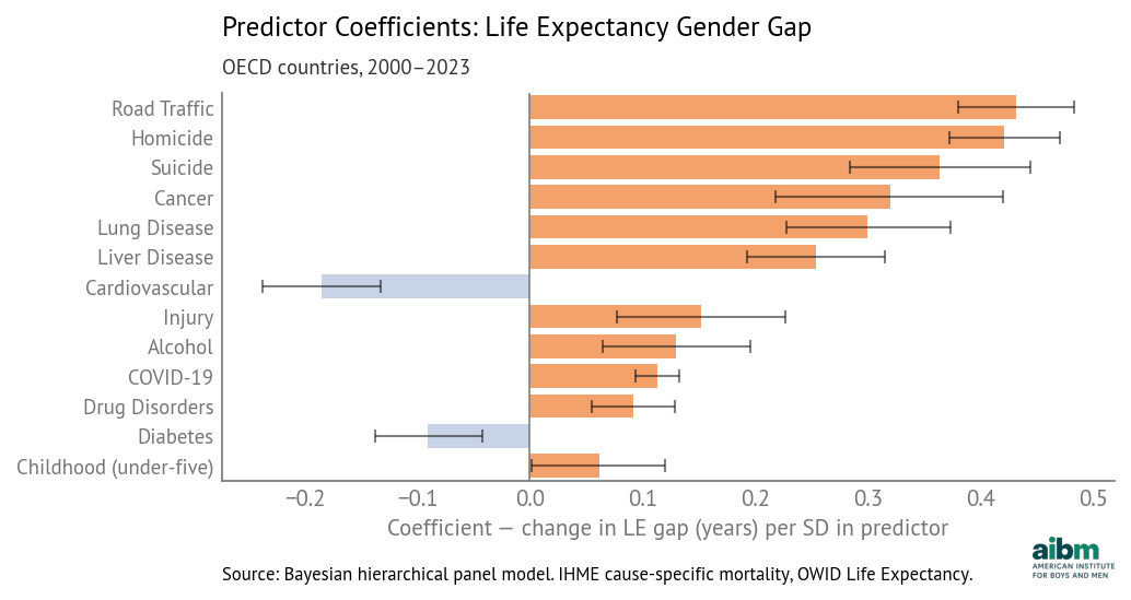
Cause of death coefficients for life expectancy gender gap (2000–2023). Source: IHME cause-specific death rates, OWID Life Expectancy, analysis by Allen Downey.
Road traffic deaths have the largest coefficient, about 0.43 years per standard deviation, which means that if a country is average in every way except that its gender gap in traffic deaths is one standard deviation above the mean, we expect its life expectancy gap to be 0.43 years above average. Other factors with large coefficients are homicide, suicide, cancer, lung disease, and liver disease.
The magnitudes of these coefficients depend on both death rates and the ages of the people affected. Cancer and respiratory disease have high rates, but they primarily affect older people, so their effect on life expectancy is attenuated. Homicide and suicide have lower rates, but they affect younger people, so their effect on life expectancy is amplified.
Child mortality affects the youngest people, so each death removes many potential years of life. But the estimated coefficient is small, and the lower bound of the credible interval is close to zero. In most OECD countries the gender gap in child mortality is already small and changes only slowly over time. So the model detects only a weak relationship between variation in child mortality and life expectancy.
The coefficient of alcohol is relatively small, but that is partly the result of classification. In the GBD database, alcohol-related deaths are defined narrowly, not including indirect effects — such as liver disease, cancer, road traffic, homicide, suicide, and accidental injury — where alcohol is often a contributing factor.
Similarly, we note the underlying effect of smoking, which contributes to gaps in death rates due to cancer, cardiovascular disease, respiratory disease, and possibly COVID-19.
Competing Risks
The coefficients for cardiovascular disease and diabetes are negative, which means that if a country has a larger death rate gap, the model predicts a smaller life expectancy gap. This is counterintuitive — for example, if more men die of cardiovascular disease, their age-specific death rates should increase and their life expectancy should decrease. So why are these two coefficients negative?
We can get a hint from the following figure, which shows the gap in death rates due to cardiovascular disease.
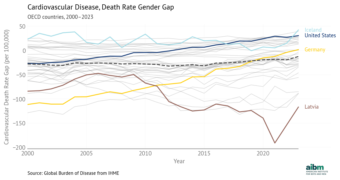
Cardiovascular disease, death rate gender gap (2000–2023), OECD countries. Source: Global Burden of Disease from IHME.
In many countries, the gap is negative, meaning that death rates from cardiovascular disease are higher for women.
Furthermore, the gap is positive (higher rates for men) in countries with the best overall health outcomes, like Iceland, and negative (higher rates for women) in countries with the worst outcomes, like Latvia. This is the opposite of the pattern we see with other causes of death, where good overall health is associated with lower death rates, which is associated with smaller gender gaps.
A possible explanation is competing risks — where death rates from other causes are low, cardiovascular disease and diabetes become more common causes of death, because they are diseases of aging. If you live long enough to die of cardiovascular disease, it means you avoided the causes of death that affect younger people.
In the regression model, these variables might act as a proxy for overall health outcomes. If a large (positive) death rate gap indicates good outcomes, and good outcomes are associated with smaller life expectancy gaps, that would explain the negative coefficients.
Importance
The magnitudes of the coefficients indicate the strength of the statistical relationship between death rate gaps and life expectancy. But they don’t tell us which factors contribute most to differences between countries and changes over time. For that, we’ll use importance, which is the product of the coefficient and the standard deviation for each cause.
We can think of the coefficient as the sensitivity of life expectancy to a hypothetical difference in death rates, and standard deviation as the size of the differences we actually see. If they are both large, the product is large. If either one is small, the product tends to be small.
The following table shows coefficients (years per SD), standard deviations, and importance for each cause.
| Cause | Standard deviation | Coefficient | Importance |
|---|---|---|---|
| Cancer | 38.2 | 0.32 [0.22, 0.421] | 12.205 [8.336, 16.025] |
| Cardiovascular disease | 36.9 | -0.185 [-0.234, -0.129] | 6.828 [4.89, 8.769] |
| Homicide | 13.5 | 0.421 [0.372, 0.469] | 5.666 [5.015, 6.333] |
| Suicide | 9.55 | 0.363 [0.28, 0.439] | 3.472 [2.718, 4.245] |
| Chronic respiratory | 10.7 | 0.299 [0.225, 0.37] | 3.21 [2.448, 4.002] |
| Road traffic | 5.91 | 0.432 [0.381, 0.484] | 2.551 [2.246, 2.857] |
| Liver disease | 9.72 | 0.254 [0.192, 0.314] | 2.469 [1.879, 3.061] |
| Unintentional injury | 15.2 | 0.152 [0.076, 0.225] | 2.309 [1.17, 3.447] |
| COVID-19 | 10.6 | 0.113 [0.093, 0.131] | 1.201 [0.995, 1.404] |
| Child mortality | 17.5 | 0.061 [-0.0, 0.116] | 1.083 [0.123, 2.095] |
| Alcohol | 6.21 | 0.13 [0.063, 0.195] | 0.808 [0.399, 1.218] |
| Diabetes | 3.53 | -0.091 [-0.136, -0.041] | 0.32 [0.15, 0.486] |
| Drug disorders | 2.79 | 0.091 [0.056, 0.13] | 0.255 [0.153, 0.359] |
The predictor with the highest coefficient, road traffic, has a relatively low standard deviation, so its importance is only moderate (6th out of 13).
The predictor with the highest importance is cancer, because it has the highest standard deviation and a moderate coefficient.
The predictor with the lowest importance is drug disorders, because it has a small coefficient and a small standard deviation.
The following figure shows the results graphically.
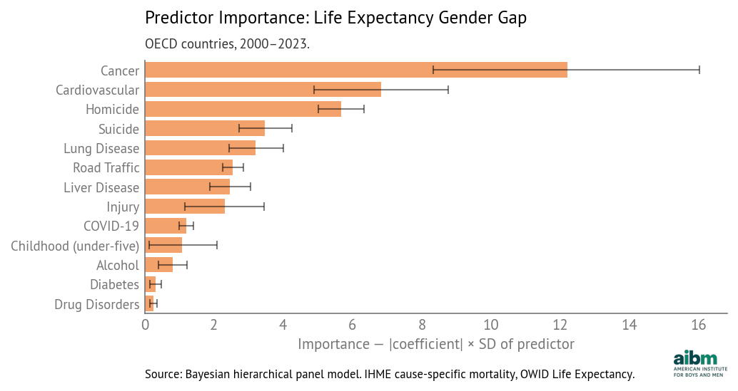
Predictor importance for life expectancy gender gap (2000–2023).
These importances direct our attention to the causes that contribute most strongly to variation in life expectancy gap:
The top three are cancer, cardiovascular disease, and homicide.
Suicide, respiratory disease, traffic, liver disease, and injury have moderate importance.
COVID-19, childhood mortality, alcohol, diabetes, and drug disorders have lower importance.
However, we should not ignore factors with lower importance.
First, the most important factor overall might not be the most important factor for a particular country. For example, drug disorders have a much larger effect on life expectancy in the United States and Canada, compared to other OECD countries. And the importance of COVID-19 is attenuated because it only affected 3 out of 24 years in the panel.
Also, some factors are easier to change than others. We might focus on a factor with only moderate importance, if we think it is more amenable to change than another factor with higher importance.
In the next post, we will look more closely at the United States to see which factors contribute most to the life expectancy gap. And we will consider which ones might be most amenable to change.
Model Details
The model uses panel data from 2000–2023 with 888 observations across 24 years and 37 OECD countries.
The model is Bayesian hierarchical regression with per-country intercepts and shared slopes. Predictors are standardized (z-scores); the target (life expectancy gap) is centered.
The model fits the data well; mean absolute error is about 0.2 years. The following figure shows residuals — the difference between actual and predicted gaps — for all 37 countries, sorted with the best-fitting countries at the top.
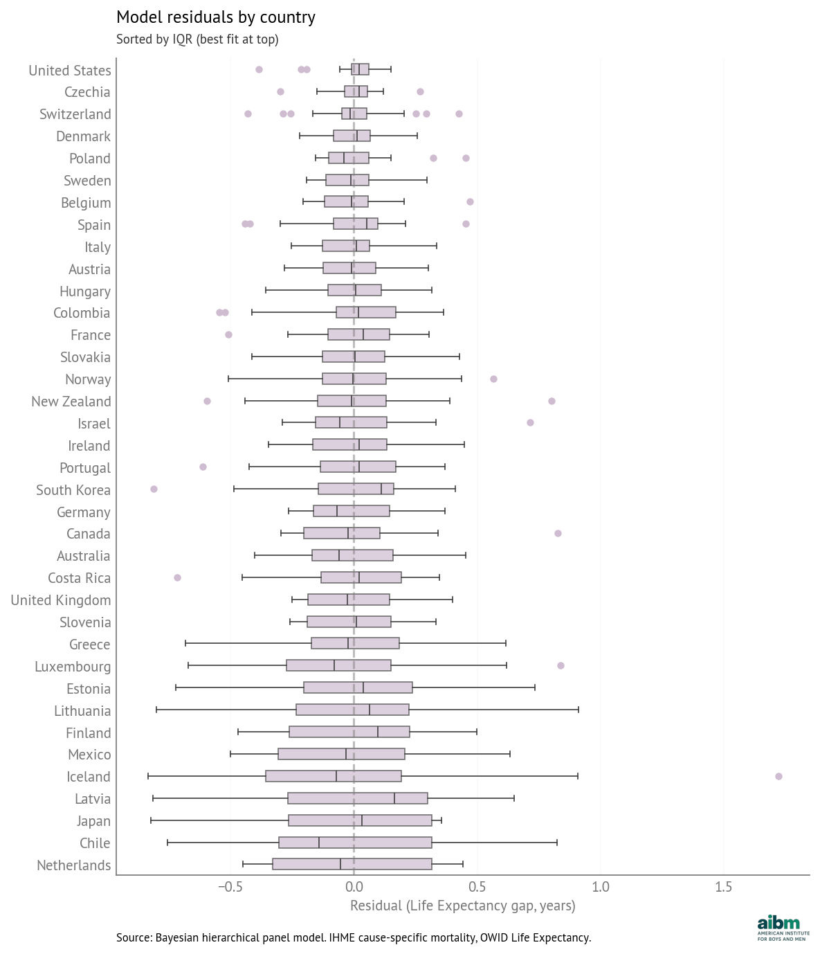
Model residuals by country (sorted by IQR, best fit at top). Source: Bayesian hierarchical panel model. IHME cause-specific mortality, OWID Life Expectancy.
The model fits some countries better than others, but even when the magnitude of the residuals is larger, they are generally centered around zero and symmetric.
To show what the quality of fit looks like, the following figure shows predicted versus actual gaps for selected countries: the United States, with the best fit, Iceland and Lithuania, with some of the worst, and France, which is near the middle. The colored lines show actual values; the gray vertical segments show 94% credible intervals for the fitted values.
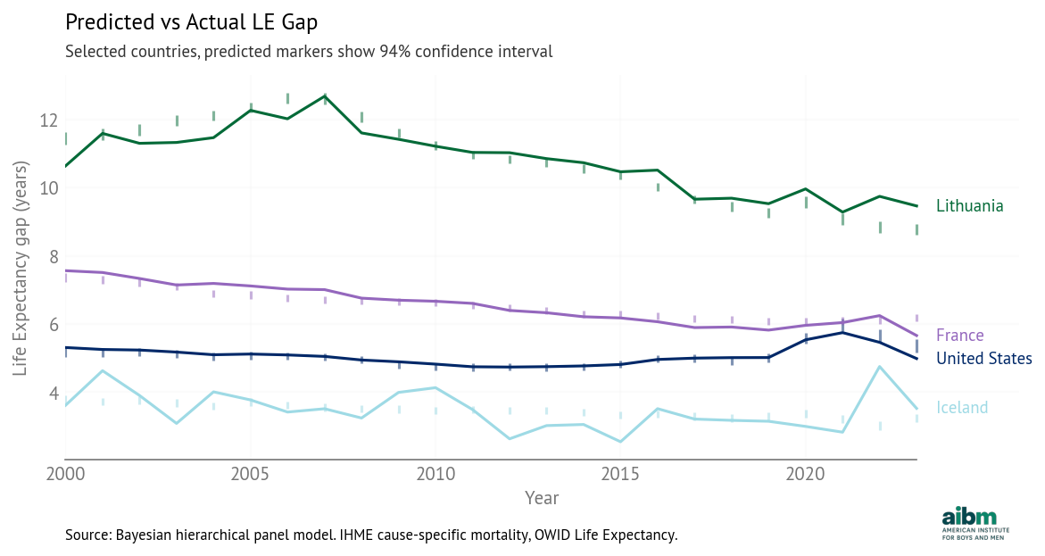
Predicted vs actual life expectancy gap (2000–2023), selected countries. Source: Bayesian hierarchical panel model. IHME cause-specific mortality, OWID Life Expectancy.
In the United States, the model tracks the observed gaps closely, including the COVID period and the opioid-driven increase. In Iceland and Lithuania, there are some large changes in the life expectancy gap that are not explained by changes in death rate gaps. Small countries might vary more over time (the United States is almost 1000 times more populous than Iceland and over 100 times more populous than Lithuania).
Variations
In addition to the 13 predictors in the model we reported, we also considered two other factors: maternal disorders and conflict/terrorism. In both cases, the estimated coefficients were small, with credible intervals that spanned zero, and the change in model fit was negligible. For both predictors, variability is small — combined with small coefficients, the resulting importances are negligible. So we removed both predictors from the model.
We exclude Turkey because when included, it appears as a statistical outlier. Turkey differs from other OECD countries in several ways — it is also possible that some of its statistics are less reliable.
As an extension to the model, we considered including death rates as well as gaps. These additional predictors improve the model fit only moderately, as they are highly correlated with the gaps — when death rates are higher, the gaps are usually higher. So adding them to the model only complicates the interpretation of the coefficients, as the effect of each cause is distributed unpredictably between the rate and the gap.
Finally, we tested a version of the model with a Gaussian Random Walk intended to capture shared temporal trends. But it complicates the model without improving fit, so we removed it for parsimony.
Next: [Counterfactuals: How much of the gap could we close?]