Rip-off ETF?#
An article in a recent issue of The Economist suggests, right in the title, “Investors should avoid a new generation of rip-off ETFs”. An ETF is an exchange-traded fund, which holds a collection of assets and trades on an exchange like a single stock. For example, the SPDR S&P 500 ETF Trust (SPY) tracks the S&P 500 index, but unlike traditional index funds, you can buy or sell shares in minutes.
There’s nothing obviously wrong with that – but as an example of a “rip-off ETF”, the article describes “defined-outcome funds” or buffer ETFs, which “offer investors an enviable-sounding opportunity: hold stocks, with protection against falling prices. All they must do is forgo annual returns above a certain level, often 10% or so.”
That might sound good, but the article explains, “Over the long term, they are a terrible deal for investors. Much of the compounding effect of stock ownership comes from rallies.”
To demonstrate, they use the value of the S&P index since 1980: “An investor with returns capped at 10% and protected from losses would have made a real return of 403% over the period, a fraction of the 3,155% return offered by just buying and holding the S&P 500.”
So that sounds bad, but returns from 1980 to the present have been historically unusual. To get a sense of whether buffer ETFs are more generally a bad deal, let’s get a bigger picture.
Click here to run this notebook on Colab
Show code cell content
from os.path import basename, exists


def download(url):
    filename = basename(url)
    if not exists(filename):
        from urllib.request import urlretrieve

        local, _ = urlretrieve(url, filename)
        print("Downloaded " + local)


download("https://github.com/AllenDowney/ThinkStats/raw/v3/nb/thinkstats.py")
Show code cell content
try:
    import empiricaldist
except ImportError:
    !pip install empiricaldist
Show code cell content
import numpy as np
import pandas as pd
import matplotlib.pyplot as plt

from thinkstats import decorate
The Dow Jones#
The MeasuringWorth Foundation has compiled the value of the Dow Jones Industrial Average at the end of each day from February 16, 1885 to the present, with adjustments at several points to make the values comparable. The series I collected starts on February 16, 1885 and ends on August 30, 2024. The following cells download and read the data.
Show code cell content
# "Citation: Samuel H. Williamson, 'Daily Closing Value of the Dow Jones Average, 1885 to Present,'
# MeasuringWorth, 2022. "

# Downloaded from https://www.measuringworth.com/datasets/DJA, September 3, 2024
DATA_PATH = "https://github.com/AllenDowney/ThinkStats/raw/v3/data/"
filename = "DJA.csv"
download(DATA_PATH + filename)
djia = pd.read_csv(filename, skiprows=4, parse_dates=[0], index_col=0)
djia.head()
| DJIA | |
|---|---|
| Date | |
| 1885-02-16 | 30.9226 |
| 1885-02-17 | 31.3365 |
| 1885-02-18 | 31.4744 |
| 1885-02-19 | 31.6765 |
| 1885-02-20 | 31.4252 |
To compute annual returns, we’ll start by selecting the closing price on the last trading day of each year (dropping 2024 because we don’t have a complete year).
annual = djia.groupby(djia.index.year).last().drop(2024)
annual
| DJIA | |
|---|---|
| Date | |
| 1885 | 39.4859 |
| 1886 | 41.2391 |
| 1887 | 37.7693 |
| 1888 | 39.5866 |
| 1889 | 42.0394 |
| ... | ... |
| 2019 | 28538.4400 |
| 2020 | 30606.4800 |
| 2021 | 36338.3000 |
| 2022 | 33147.2500 |
| 2023 | 37689.5400 |
139 rows × 1 columns
Next we’ll compute the annual price return, which is the ratio of successive year-end closing prices.
annual['Ratio'] = annual['DJIA'] / annual['DJIA'].shift(1)
annual
| DJIA | Ratio | |
|---|---|---|
| Date | ||
| 1885 | 39.4859 | NaN |
| 1886 | 41.2391 | 1.044401 |
| 1887 | 37.7693 | 0.915861 |
| 1888 | 39.5866 | 1.048116 |
| 1889 | 42.0394 | 1.061960 |
| ... | ... | ... |
| 2019 | 28538.4400 | 1.223384 |
| 2020 | 30606.4800 | 1.072465 |
| 2021 | 36338.3000 | 1.187275 |
| 2022 | 33147.2500 | 0.912185 |
| 2023 | 37689.5400 | 1.137034 |
139 rows × 2 columns
And the relative return as a percentage.
annual['Return'] = (annual['Ratio'] - 1) * 100
Looking at the years with the biggest losses and gains, we can see that most of the extremes were before the 1960s – with the exception of the 2008 financial crisis.
annual.dropna().sort_values(by='Return')
| DJIA | Ratio | Return | |
|---|---|---|---|
| Date | |||
| 1931 | 77.9000 | 0.473326 | -52.667396 |
| 1907 | 43.0382 | 0.622683 | -37.731743 |
| 2008 | 8776.3900 | 0.661629 | -33.837097 |
| 1930 | 164.5800 | 0.662347 | -33.765293 |
| 1920 | 71.9500 | 0.670988 | -32.901240 |
| ... | ... | ... | ... |
| 1954 | 404.3900 | 1.439623 | 43.962264 |
| 1908 | 63.1104 | 1.466381 | 46.638103 |
| 1928 | 300.0000 | 1.482213 | 48.221344 |
| 1933 | 99.9000 | 1.666945 | 66.694477 |
| 1915 | 99.1500 | 1.816599 | 81.659949 |
138 rows × 3 columns
Here’s what the distribution of annual returns looks like.
from empiricaldist import Cdf

cdf_return = Cdf.from_seq(annual['Return'])
cdf_return.plot()

decorate(xlabel='Annual return (percent)', ylabel='CDF')
plt.savefig('ripoff_etf1.png', dpi=300)
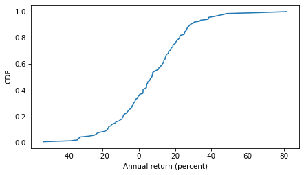
Immediately we see why capping returns at 10% might be a bad idea – this cap is exceeded almost 45% of the time, and sometimes by a lot!
1 - cdf_return(10)
0.4492753623188406
Long-Term Returns#
We’ll use the following function to compute long-term returns. It takes a start date and a duration, and computes two ratios:
The total price return based on actual annual returns.
The total price return if annual returns are clipped at 0 and 10 – that is, any negative returns are set to 0 and any returns above 10 are set to 10.
def compute_ratios(start=1993, duration=30):
    end = start + duration
    interval = annual.loc[start: end]
    ratio = interval['Ratio'].prod()
    low, high = 1.0, 1.10
    clipped = interval['Ratio'].clip(low, high)
    ratio_clipped = clipped.prod()
    return start, end, ratio, ratio_clipped
With this function, we can replicate the analysis The Economist did with the S&P 500. Here are the results for the DJIA from the beginning of 1980 to the end of 2023.
compute_ratios(1980, 43)
(1980, 2023, 44.93751117788029, 15.356490985533199)
A buffer ETF over this period would have grown by a factor of more than 15 in nominal dollars, with no risk of loss. But an index fund would have grown by a factor of almost 45. So yeah, the ETF would have been a bad deal.
However, if we go back to the bad old days, an investor in 1900 would have been substantially better off with a buffer ETF held for 43 years – a factor of 7.2 compared to a factor of 2.8.
compute_ratios(1900, 43)
(1900, 1943, 2.8071864303140583, 7.225624631784611)
It seems we can cherry-pick the data to make the comparison go either way – so let’s see how things look more generally. Starting in 1886, we’ll compute price returns for all 30-year intervals, ending with the interval from 1993 to 2023.
duration = 30
ratios = [compute_ratios(start, duration) for start in range(1886, 2024-duration)]
ratios = pd.DataFrame(ratios, columns=['Start', 'End', 'Index Fund', 'Buffer ETF'])
ratios.index = ratios['Start']
ratios.tail()
| Start | End | Index Fund | Buffer ETF | |
|---|---|---|---|---|
| Start | ||||
| 1989 | 1989 | 2019 | 13.160027 | 6.532125 |
| 1990 | 1990 | 2020 | 11.116693 | 6.368615 |
| 1991 | 1991 | 2021 | 13.797643 | 7.005476 |
| 1992 | 1992 | 2022 | 10.460407 | 6.368615 |
| 1993 | 1993 | 2023 | 11.417232 | 6.724757 |
Here’s what the returns look like for an index fund compared to a buffer ETF.
ratios['Index Fund'].plot()
ratios['Buffer ETF'].plot()

decorate(xlabel='Start year', ylabel='30-year price return')
plt.savefig('ripoff_etf2.png', dpi=300)
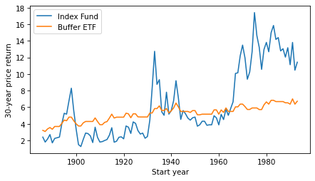
The buffer ETF performs as advertised, substantially reducing volatility. But it has only occasionally been a good deal, and not in my lifetime.
According to ChatGPT, the primary reasons for strong growth in stock prices since the 1960s are “technological advancements, globalization, financial market innovation, and favorable monetary policies”. If you think these elements will generally persist over the next 30 years, you might want to avoid buffer ETFs.