The third edition of Think Stats is not for sale yet, but if you would like to support this project, you can buy me a coffee.

6. Probability Density Functions

In the previous chapter, we modeled data with theoretical distributions including the binomial, Poisson, exponential, and normal distributions.

The binomial and Poisson distributions are discrete, which means that the outcomes have to be distinct or separate elements, like an integer number of hits and misses, or goals scored. In a discrete distribution, each outcome is associated with a probability mass.

The exponential and normal distribution are continuous, which means the outcomes can be locations on a spectrum – like a wavelength – or ratios – like height and weight, which are ratios relative to their units of measure. In a discrete distribution, each outcome is associated with a probability density. Probability density is an abstract idea, and many people find it difficult at first, but we’ll take it one step at a time. As a first step, let’s think again about comparing distributions.

Click here to run this notebook on Colab.

Show code cell content Hide code cell content

from os.path import basename, exists


def download(url):
    filename = basename(url)
    if not exists(filename):
        from urllib.request import urlretrieve

        local, _ = urlretrieve(url, filename)
        print("Downloaded " + local)


download("https://github.com/AllenDowney/ThinkStats/raw/v3/nb/thinkstats.py")

Show code cell content Hide code cell content

try:
    import empiricaldist
except ImportError:
    !pip install empiricaldist

Show code cell content Hide code cell content

import numpy as np
import pandas as pd
import matplotlib.pyplot as plt

from thinkstats import decorate

6.1. Comparing Distributions

In the previous chapter, when we compared discrete distributions, we used a bar plot to show their probability mass functions (PMFs). When we compared continuous distributions, we used a line plot to show their cumulative distribution functions (CDFs).

For the discrete distributions, we could also have used CDFs. For example, here’s the PMF of a Poisson distribution with parameter lam=2.2, which is a good model for the distribution of household size in the NSFG data.

The following cells download the data files and install statadict, which we need to read the data.

download("https://github.com/AllenDowney/ThinkStats/raw/v3/nb/nsfg.py")
download("https://github.com/AllenDowney/ThinkStats/raw/v3/data/2002FemResp.dct")
download("https://github.com/AllenDowney/ThinkStats/raw/v3/data/2002FemResp.dat.gz")

try:
    import statadict
except ImportError:
    !pip install statadict

We can use read_fem_resp to read the respondent data file.

from nsfg import read_fem_resp

resp = read_fem_resp()

Next we’ll select household sizes for people 25 and older.

older = resp.query("age >= 25")
num_family = older["numfmhh"]

And make a Pmf that represents the distribution of responses.

from empiricaldist import Pmf

pmf_family = Pmf.from_seq(num_family, name="data")

Here’s another Pmf that represents a Poisson distribution with the same mean.

from thinkstats import poisson_pmf

lam = 2.2
ks = np.arange(11)
ps = poisson_pmf(ks, lam)

pmf_poisson = Pmf(ps, ks, name="Poisson model")

And here’s how the distribution of the data compares to the Poisson model.

from thinkstats import two_bar_plots

two_bar_plots(pmf_family, pmf_poisson)
decorate(xlabel="Number of family members")

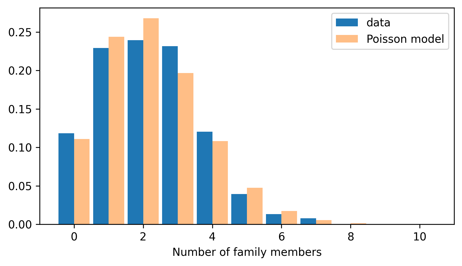
Comparing the PMFs, we can see that the model fits the data well, but with some deviations.

To get a sense of how substantial those deviations are, it can be helpful to compare CDFs. We can use make_cdf to compute the CDFs of the data and the model.

cdf_family = pmf_family.make_cdf()
cdf_poisson = pmf_poisson.make_cdf()

Here’s what they look like.

from thinkstats import two_cdf_plots

two_cdf_plots(cdf_poisson, cdf_family)
decorate(xlabel="Number of family members")

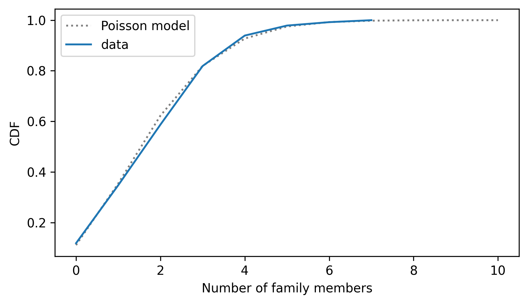
When we compare CDFs, the deviations are less prominent, but we can see where and how the distributions differ. PMFs tend to emphasize small differences – sometimes CDFs provide a better sense of the big picture.

CDFs also work well with continuous data. As an example, let’s look at the distribution of birth weights again, which is in the NSFG pregnancy file.

download("https://github.com/AllenDowney/ThinkStats/raw/v3/data/2002FemPreg.dct")
download("https://github.com/AllenDowney/ThinkStats/raw/v3/data/2002FemPreg.dat.gz")

from nsfg import read_fem_preg

preg = read_fem_preg()
birth_weights = preg["totalwgt_lb"].dropna()

Here is the code we used in the previous chapter to fit a normal model to the data.

from scipy.stats import trimboth
from thinkstats import make_normal_model

trimmed = trimboth(birth_weights, 0.01)
cdf_model = make_normal_model(trimmed)

And here’s the distribution of the data compared to the normal model.

from empiricaldist import Cdf

cdf_birth_weight = Cdf.from_seq(birth_weights, name="sample")
two_cdf_plots(cdf_model, cdf_birth_weight, xlabel="Birth weight (pounds)")

As we saw in the previous chapter, the normal model fits the data well except in the range of the lightest babies.

In my opinion, CDFs are usually the best way to compare data to a model. But for audiences that are not familiar with CDFs, there is one more option: probability density functions.

6.2. Probability Density

We’ll start with the probability density function (PDF) of the normal distribution, which computes the density for the quantities, xs, given the parameters mu and sigma.

def normal_pdf(xs, mu, sigma):
    """Evaluates the normal probability density function."""
    z = (xs - mu) / sigma
    return np.exp(-(z**2) / 2) / sigma / np.sqrt(2 * np.pi)

For the parameters mu and sigma, we’ll use the mean and standard deviation of the trimmed birth weights.

m, s = np.mean(trimmed), np.std(trimmed)

Now we’ll evaluate normal_pdf for a range of weights.

low = m - 4 * s
high = m + 4 * s
qs = np.linspace(low, high, 201)
ps = normal_pdf(qs, m, s)

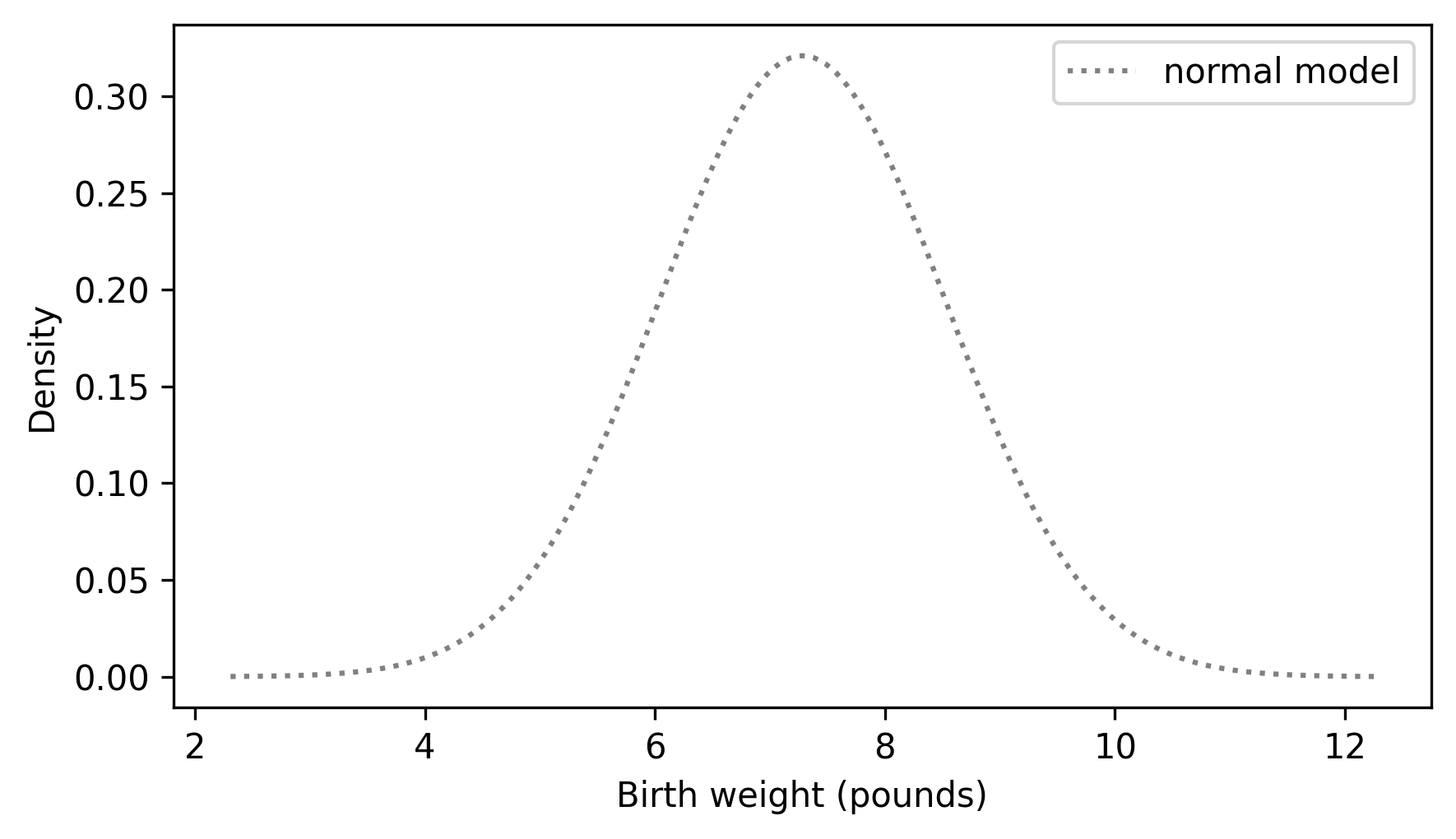
The result looks like a bell curve, which is characteristic of the normal distribution.

plt.plot(qs, ps, label="normal model")
decorate(xlabel="Birth weight (pounds)", ylabel="Density")

When we evaluate normal_pdf, the result is a probability density. For example, here’s the density function evaluated at the mean, which is where the density is highest.

normal_pdf(m, m, s)

0.32093416297880123

By itself, a probability density doesn’t mean much – most importantly, it is not a probability. It would be incorrect to say that the probability is 32% that a randomly-chosen birth weight equals m. In fact, the probability that a birth weight is truly, exactly, and precisely equal to m – or any other specific value – is effectively zero.

However, we can use these probability densities to compute the probability that a birth weight falls in an interval between two values, by computing the area under the curve.

We can do that with the normal_pdf function, but it will be more convenient to use a NormalPdf object, which is defined in the thinkstats module. Here’s how we can use it to create a NormalPdf with the same mean and standard deviation as the birth weights in the NSFG dataset.

from thinkstats import NormalPdf

pdf_model = NormalPdf(m, s, name="normal model")
pdf_model

NormalPdf(7.280883100022579, 1.2430657948614345, name='normal model')

If we call this object like a function, it evaluates the normal PDF.

pdf_model(m)

0.32093416297880123

Now, to compute the area under the PDF, we can use the following function, which takes a NormalPdf object and the bounds of an interval, low and high. It evaluates the normal PDF at equally-spaced quantities between low and high, and uses Simpson’s method to estimate the area under the curve.

from scipy.integrate import simpson


def area_under(pdf, low, high):
    """Find the area under a PDF.

    pdf: Pdf object
    low: low end of the interval
    high: high end of the interval
    """
    qs = np.linspace(low, high, 501)
    ps = pdf(qs)
    return simpson(y=ps, x=qs)

If we compute the area under the curve from the lowest to the highest point in the graph, the result is close to 1.

area_under(pdf_model, 2, 12)

0.9999158086616793

If we extend the interval from negative infinity to positive infinity, the total area is exactly 1.

If we start from 0 – or any value far below the mean – we can compute the fraction of birth weights less than or equal to 8.5 pounds.

area_under(pdf_model, 0, 8.5)

0.8366380335513807

You might recall that the “fraction less than or equal to a given value” is the definition of the CDF. So we could compute the same result using the CDF of the normal distribution.

from scipy.stats import norm

norm.cdf(8.5, m, s)

0.8366380358092718

Similarly, we can use the area under the density curve to compute the fraction of birth weights between 6 and 8 pounds.

area_under(pdf_model, 6, 8)

0.5671317752927691

Or we can get the same result using the CDF to compute the fraction less than 8 and then subtracting off the fraction less than 6.

norm.cdf(8, m, s) - norm.cdf(6, m, s)

0.5671317752921801

So the CDF is the area under the curve of the PDF. If you know calculus, another way to say the same thing is that the CDF is the integral of the PDF. And conversely, the PDF is the derivative of the CDF.

6.3. The Exponential PDF

To get your head around probability density, it might help to see another example. In the previous chapter, we used an exponential distribution to model the time until the first goal in a hockey game. We used the following function to compute the exponential CDF, where lam is the rate parameter in goals per unit of time.

def exponential_cdf(x, lam):
    """Compute the exponential CDF.

    x: float or sequence of floats
    lam: rate parameter

    returns: float or NumPy array of cumulative probability
    """
    return 1 - np.exp(-lam * x)

We can compute the PDF of the exponential distribution like this.

def exponential_pdf(x, lam):
    """Evaluates the exponential PDF.

    x: float or sequence of floats
    lam: rate parameter

    returns: float or NumPy array of probability density
    """
    return lam * np.exp(-lam * x)

thinkstats provides an ExponentialPdf object that uses this function to compute the exponential PDF. We can use one to represent an exponential distribution with rate parameter 6 goals per game.

from thinkstats import ExponentialPdf

lam = 6
pdf_expo = ExponentialPdf(lam, name="model")
pdf_expo

ExponentialPdf(6, name='model')

ExponentialPdf provides a plot function we can use to plot the PDF – notice that the unit of time is games here, rather than seconds as in the previous chapter.

qs = np.linspace(0, 1.5, 201)
pdf_expo.plot(qs)
decorate(xlabel="Time (games)", ylabel="Density")

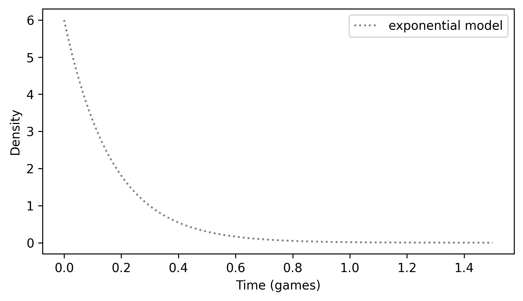
Looking at the y-axis, you might notice that some of these densities are greater than 1, which is a reminder that a probability density is not a probability. But the area under a density curve is a probability, so it should never be greater than 1.

If we compute the area under this curve from 0 to 1.5 games, we can confirm that the result is close to 1.

area_under(pdf_expo, 0, 1.5)

0.999876590779019

If we extend the interval much farther, the result is slightly greater than 1, but that’s because we’re approximating the area numerically. Mathematically, it is exactly 1, as we can confirm using the exponential CDF.

from thinkstats import exponential_cdf

exponential_cdf(7, lam)

1.0

We can use the area under the density curve to compute the probability of a goal during any interval. For example, here is the probability of a goal during the first minute of a 60-minute game.

area_under(pdf_expo, 0, 1 / 60)

0.09516258196404043

We can compute the same result using the exponential CDF.

exponential_cdf(1 / 60, lam)

0.09516258196404048

In summary, if we evaluate a PDF, the result is a probability density – which is not a probability. However, if we compute the area under the PDF, the result is the probability that a quantity falls in an interval. Or we can find the same probability by evaluating the CDF at the beginning and end of the interval and computing the difference.

6.4. Comparing PMFs and PDFs

It is a common error to compare the PMF of a sample with the PDF of a theoretical model. For example, suppose we want to compare the distribution of birth weights to a normal model. Here’s a Pmf that represents the distribution of the data.

pmf_birth_weight = Pmf.from_seq(birth_weights, name="data")

And we already have pdf_model, which represents the PDF of the normal distribution with the same mean and standard deviation. Here’s what happens if we plot them on the same axis.

pmf_birth_weight.plot()
pdf_model.plot(color="gray")

decorate(xlabel="Birth weight (pounds)", ylabel="PMF? Density?")

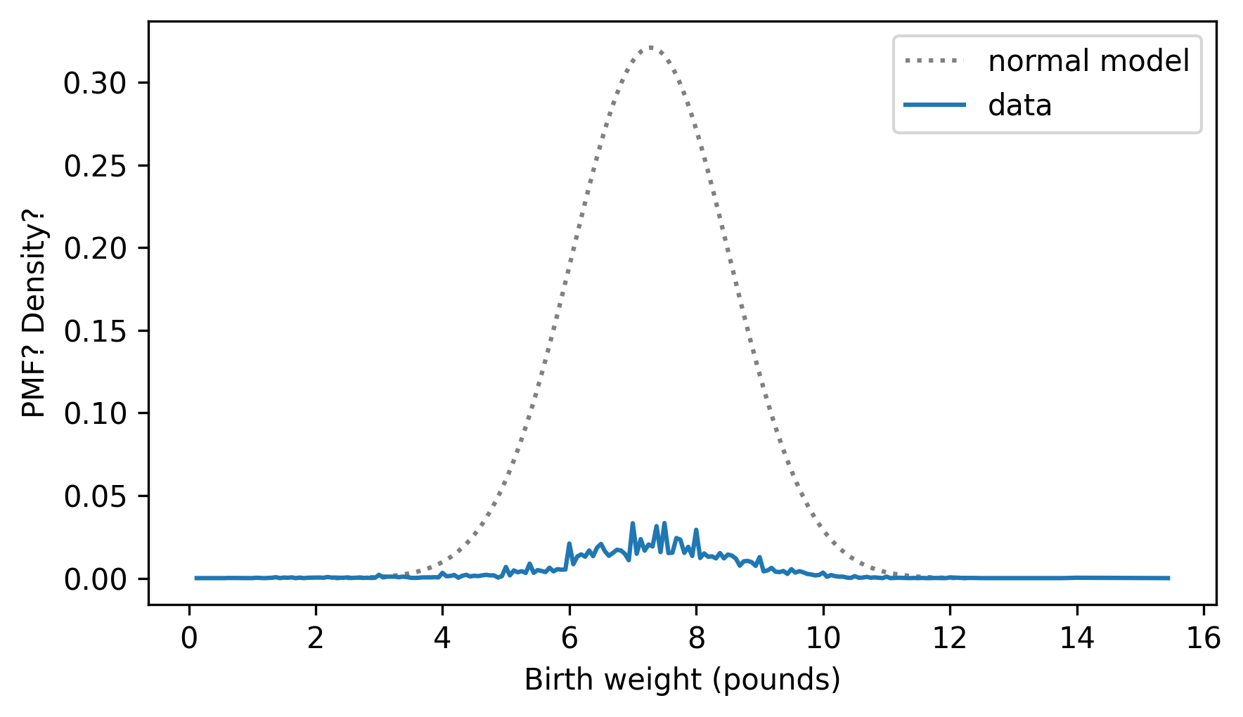
It doesn’t work very well. One reason is that they are not in the same units. A PMF contains probability masses and a PDF contains probability densities, so we can’t compare them, and we shouldn’t plot them on the same axes.

As a first attempt to solve the problem, we can make a Pmf that approximates the normal distribution by evaluating the PDF at a discrete set of points. NormalPdf provides a make_pmf method that does that.

pmf_model = pdf_model.make_pmf()

The result contain probability masses, so we can at least plot it on the same axes as the PMF of the data.

pmf_model.plot(color="gray")
pmf_birth_weight.plot()

decorate(xlabel="Birth weight (pounds)", ylabel="PMF")

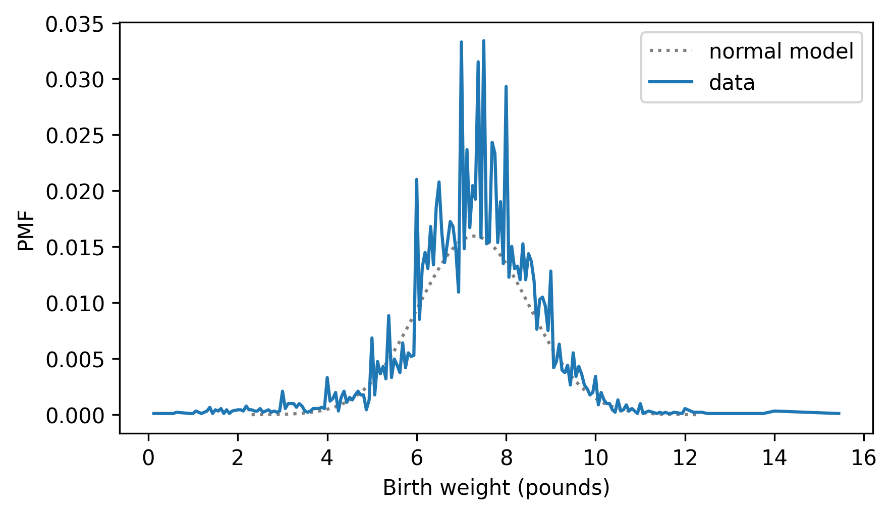
But this is still not a good way to compare distributions. One problem is that the two Pmf objects contains different numbers of quantities, and the quantities in pmf_birth_weight are not equally spaced, so the probability masses are not really comparable.

len(pmf_model), len(pmf_birth_weight)

(201, 184)

The other problem is that the Pmf of the data is noisy. So let’s try something else.

6.5. Kernel Density Estimation

Instead of converting the model to a PMF, we can convert the distribution of the data to a PDF. To show how that works, I’ll start with a small sample of the data.

# Set the random seed so we get the same results every time
np.random.seed(3)

n = 10
sample = birth_weights.sample(n)

The Pmf of this sample looks like this.

for weight in sample:
    pmf = Pmf.from_seq([weight]) / n
    pmf.bar(width=0.08, alpha=0.5)

xlim = [1.5, 12.5]
decorate(xlabel="Birth weight (pounds)", ylabel="PMF", xlim=xlim)

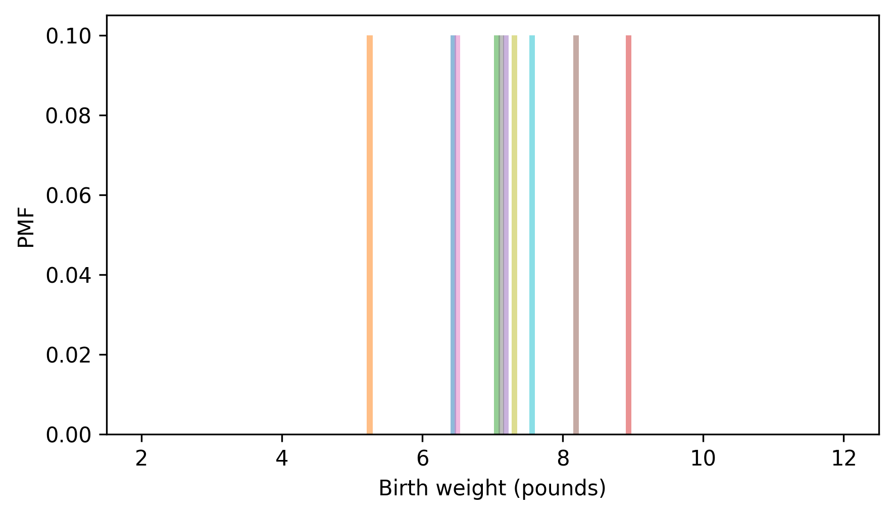
This way of representing the distribution treats the data as if it is discrete, so each probability mass is stacked up on a single point. But birth weight is actually continuous, so the quantities between the measurements are also possible. We can represent that possibility by replacing each discrete probability mass with a continuous probability density, like this.

qs = np.linspace(2, 12, 201)

for weight in sample:
    ps = NormalPdf(weight, 0.75)(qs) / n
    plt.plot(qs, ps, alpha=0.5)

decorate(xlabel="Birth weight (pounds)", ylabel="PDF", xlim=xlim)

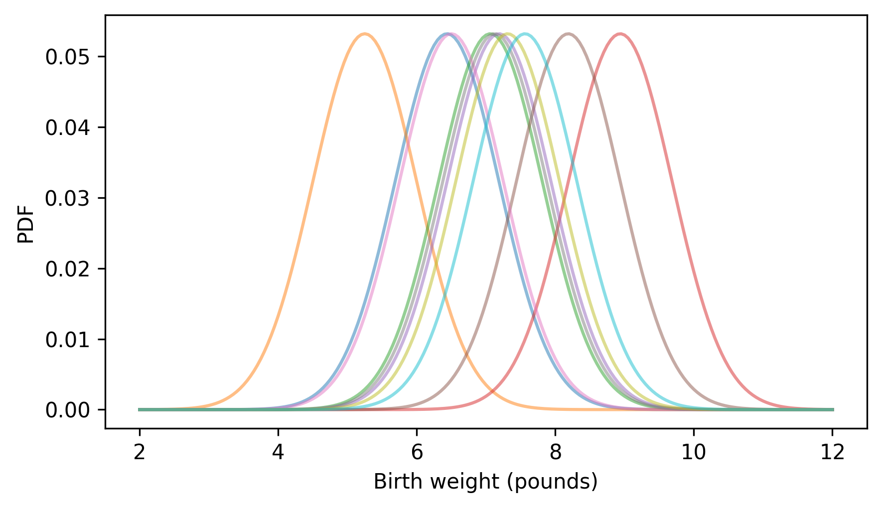
For each weight in the sample, we create a NormalPdf with the observed weight as the mean – now let’s add them up.

low_ps = np.zeros_like(qs)

for weight in sample:
    ps = NormalPdf(weight, 0.75)(qs) / n
    high_ps = low_ps + ps
    plt.fill_between(qs, low_ps, high_ps, alpha=0.5, lw=1, ec="white")
    low_ps = high_ps

decorate(xlabel="Birth weight (pounds)", ylabel="PDF", xlim=xlim)

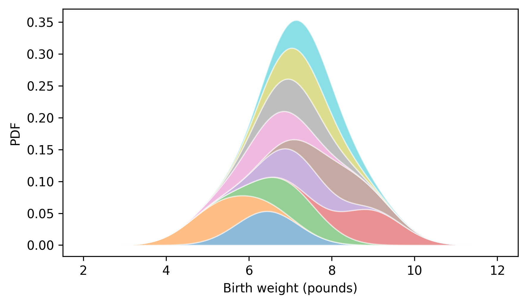
When we add up the probability densities for each data point, the result is an estimate of the probability density for the whole sample. This process is called kernel density estimation or KDE. In this context, a “kernel” is one of the small density functions we added up. Because the kernels we used are normal distributions – also known as Gaussians – we could say more specifically that we computed a Gaussian KDE.

SciPy provides a function called gaussian_kde that implements this algorithm. Here’s how we can use it to estimate the distribution of birth weights.

from scipy.stats import gaussian_kde

kde = gaussian_kde(birth_weights)

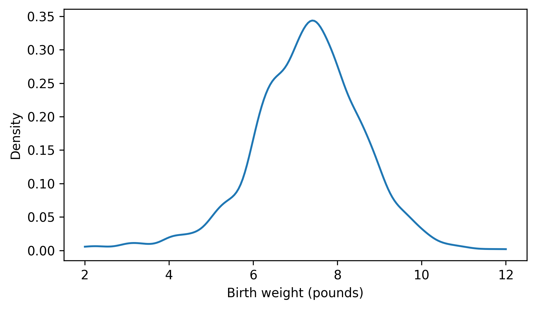
The result is an object that represents the estimated PDF, which we can evaluate by calling it like a function.

ps = kde(qs)

Here’s what the result looks like.

plt.plot(qs, ps)

decorate(xlabel="Birth weight (pounds)", ylabel="Density")

thinkstats provides a Pdf object that takes the result from gaussian_kde, and a domain that indicates where the density should be evaluated. Here’s how we make one.

from thinkstats import Pdf

domain = np.min(birth_weights), np.max(birth_weights)
kde_birth_weights = Pdf(kde, domain, name="data")

Pdf provides a plot method we can use to compare the estimated PDF of the sample to the PDF of a normal distribution.

kde_birth_weights.plot()
pdf_model.plot(color="gray")

decorate(xlabel="Birth weight (pounds)", ylabel="Density")

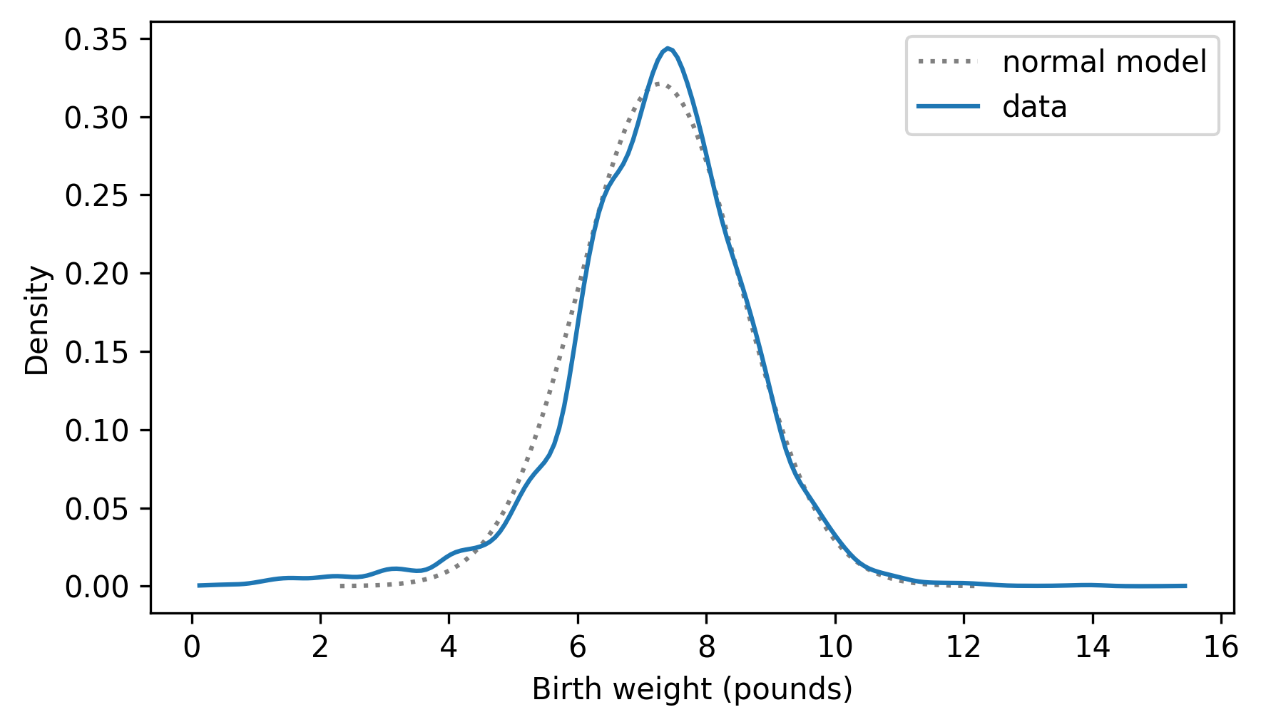
Kernel density estimation makes it possible to compare the distribution of a dataset to a theoretical model, and for some audiences, this is a good way to visualize the comparison. But for audiences that are familiar with CDFs, I think comparing CDFs are usually better.

6.6. The Distribution Framework

At this point we have a complete set of ways to represent distributions: PMFs, CDFs, and PDFs The following figure shows these representations and the transitions from one to another. For example, if we have a Pmf, we can use the cumsum function to compute the cumulative sum of the probabilities and get a Cdf that represents the same distribution.

To demonstrate these transitions, we’ll use a new dataset that “contains the time of birth, sex, and birth weight for each of 44 babies born in one 24-hour period at a Brisbane, Australia, hospital.” Instructions for downloading the data are in the notebook for this chapter.

According to the information in the file

Source: Steele, S. (December 21, 1997), “Babies by the Dozen for Christmas: 24-Hour Baby Boom,” The Sunday Mail (Brisbane), p. 7.

STORY BEHIND THE DATA: Forty-four babies – a new record – were born in one 24-hour period at the Mater Mothers’ Hospital in Brisbane, Queensland, Australia, on December 18, 1997. For each of the 44 babies, The Sunday Mail recorded the time of birth, the sex of the child, and the birth weight in grams.

Additional information about this dataset can be found in the “Datasets and Stories” article “A Simple Dataset for Demonstrating Common Distributions” in the Journal of Statistics Education (Dunn 1999).

Downloaded from https://jse.amstat.org/datasets/babyboom.txt

download("https://github.com/AllenDowney/ThinkStats/raw/v3/data/babyboom.dat")

We can read the data like this.

from thinkstats import read_baby_boom

boom = read_baby_boom()
boom.head()

	time	sex	weight_g	minutes
0	5	1	3837	5
1	104	1	3334	64
2	118	2	3554	78
3	155	2	3838	115
4	257	2	3625	177

The minutes column records “the number of minutes since midnight for each birth”. So can use the diff method to compute the interval between each successive birth.

diffs = boom["minutes"].diff().dropna()

If births happen with equal probability during any minute of the day, we expect these intervals to follow an exponential distribution. In reality, that assumption is not precisely true, but the exponential distribution might still be a good model for the data.

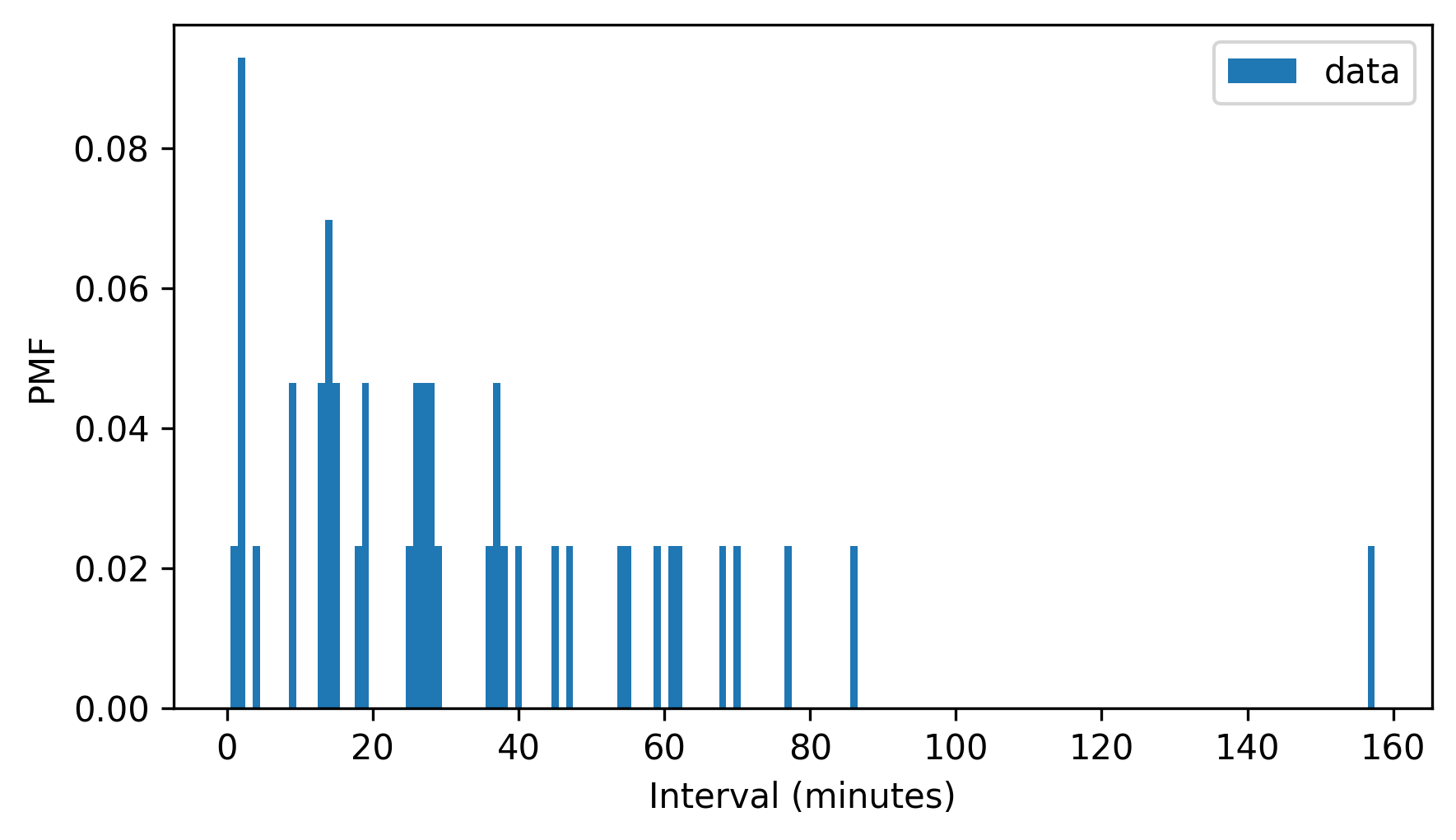
To find out, we’ll start by making a Pmf that represents the distribution of intervals.

pmf_diffs = Pmf.from_seq(diffs, name="data")
pmf_diffs.bar(width=1)

decorate(xlabel="Interval (minutes)", ylabel="PMF")

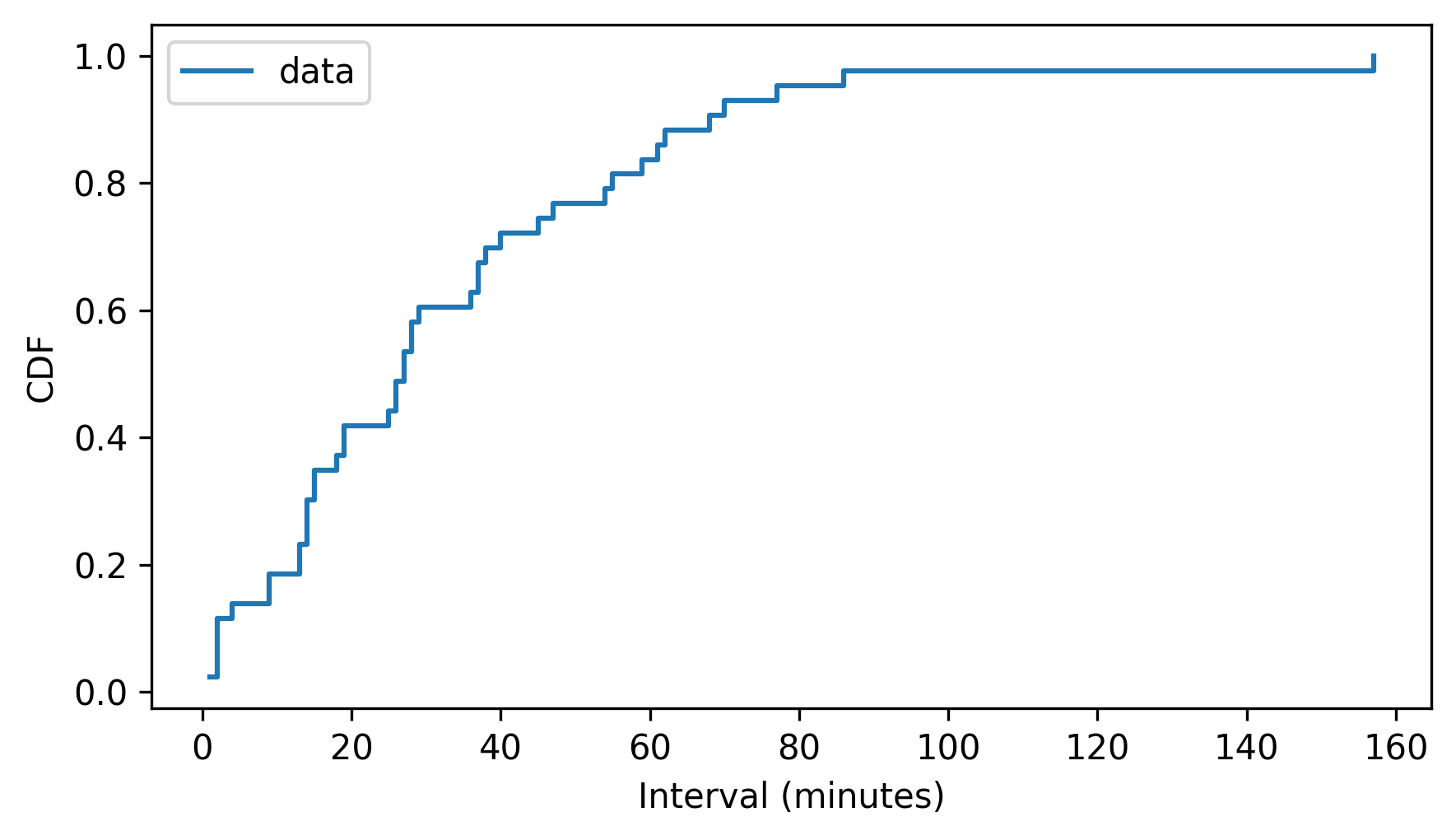
Then we can use make_cdf to compute the cumulative probabilities and store them in a Cdf object.

cdf_diffs = pmf_diffs.make_cdf()
cdf_diffs.step(color="C1")

decorate(xlabel="Interval (minutes)", ylabel="CDF")

The Pmf and Cdf are equivalent in the sense that if we are given either one, we can compute the other. To demonstrate, we’ll use the make_pmf method, which computes the differences between successive probabilities in a Cdf and returns a Pmf.

pmf_diffs2 = cdf_diffs.make_pmf()

The result should be identical to the original Pmf, but there might be small floating-point errors. We can use allclose to check that the result is close to the original Pmf.

np.allclose(pmf_diffs, pmf_diffs2)

True

And it is.

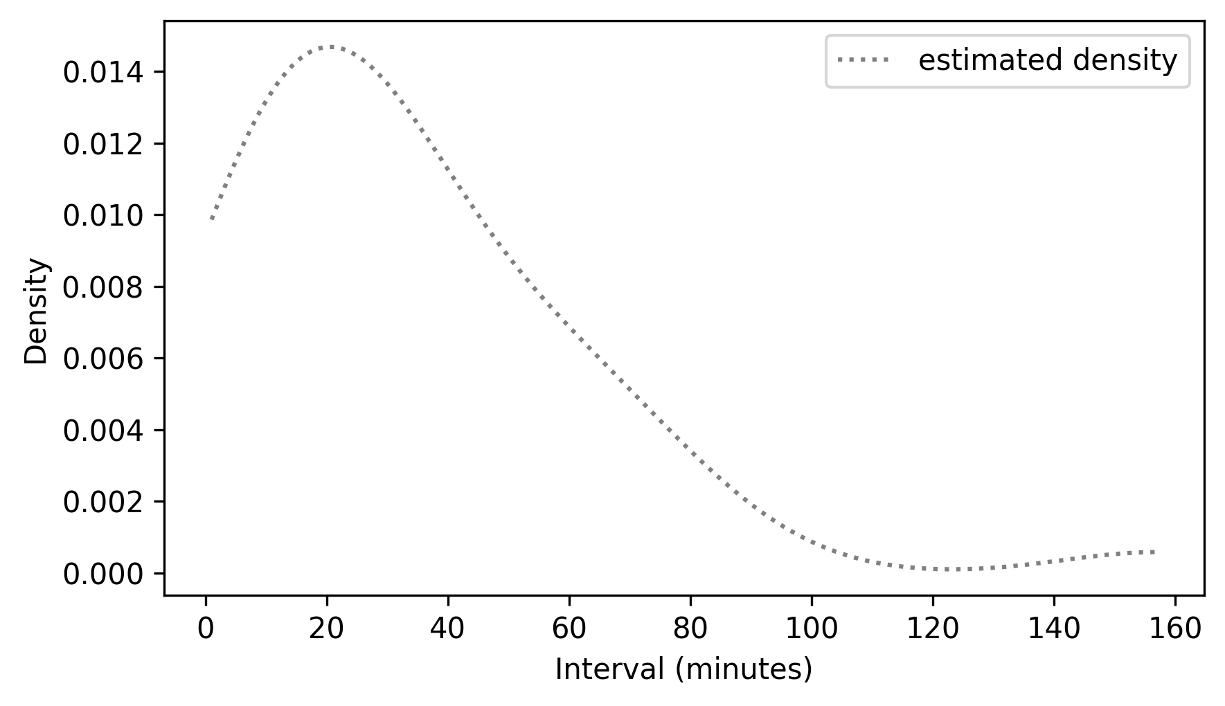
From a Pmf, we can estimate a density function by calling gaussian_kde with the probabilities from the Pmf as weights.

kde = gaussian_kde(pmf_diffs.qs, weights=pmf_diffs.ps)

To plot the results, we can use kde to make Pdf object, and call the plot method.

domain = np.min(pmf_diffs.qs), np.max(pmf_diffs.qs)
kde_diffs = Pdf(kde, domain=domain, name="estimated density")

kde_diffs.plot()
decorate(xlabel="Interval (minutes)", ylabel="Density")

To see whether the estimated density follows an exponential model, we can make an ExponentialPdf with the same mean as the data.

m = diffs.mean()
lam = 1 / m
pdf_model = ExponentialPdf(lam, name="exponential PDF")

Here’s what it looks like compared to the estimated density.

pdf_model.plot(color="gray")
kde_diffs.plot()
decorate(xlabel="Interval (minutes)", ylabel="Density")

Comparing the estimated density to an exponential PDF, it doesn’t seem like the model fits the data well. But that might be misleading – again, I think comparing CDFs provides the clearer picture.

Here’s the CDF of an exponential distribution compared to the CDF of the data.

from thinkstats import ExponentialCdf

cdf_model = ExponentialCdf(lam, name="exponential CDF")
cdf_model.plot(color="gray")
cdf_diffs.step(color="C1")

decorate(xlabel="Interval (minutes)", ylabel="CDF")

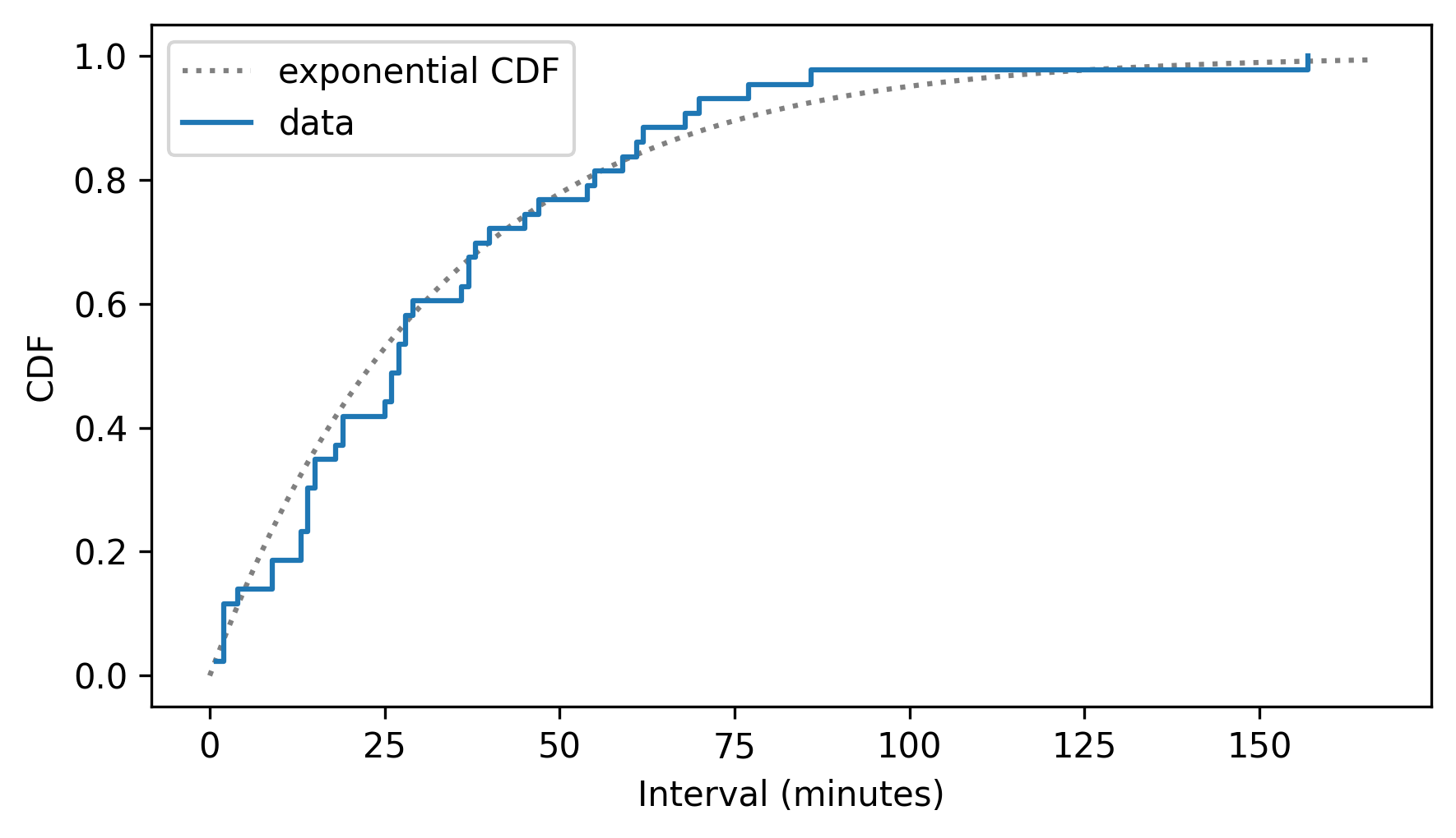
The exponential model fits the CDF of the data well.

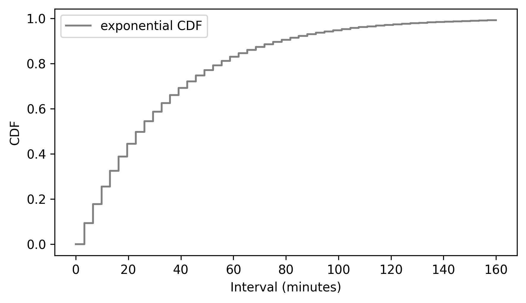
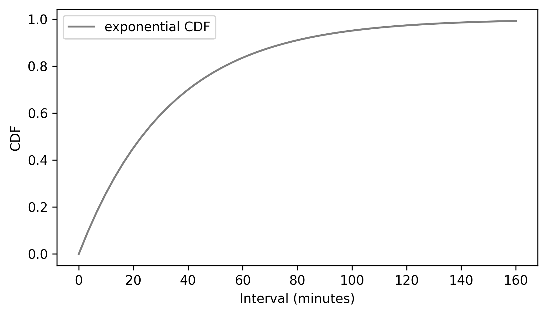
Given an ExponentialPdf, we can use make_pmf to discretize the PDF – that is, to make a discrete approximation by evaluating the PDF at a sequence of equally spaced quantities.

qs = np.linspace(0, 175, 31)
pmf_model = pdf_model.make_pmf(qs)
pmf_model.bar(width=2)

decorate(xlabel="Interval (minutes)", ylabel="PMF")

And given an ExponentialCdf, we can use make_cdf to make a discrete approximation of the exponential CDF.

discrete_cdf_model = cdf_model.make_cdf(qs)
discrete_cdf_model.step()

decorate(xlabel="Interval (minutes)", ylabel="CDF")

Finally, to get from a discrete CDF to a continuous CDF, we can interpolate between the steps, which is what we see if we use the plot method instead of the step method.

discrete_cdf_model.plot()

decorate(xlabel="Interval (minutes)", ylabel="CDF")

Finally, a PDF is the derivative of a continuous CDF, and a CDF is the integral of a PDF.

To demonstrate, we can use SymPy to define the CDF of an exponential distribution and compute its derivative.

import sympy as sp

x = sp.Symbol("x", real=True, positive=True)
λ = sp.Symbol("λ", real=True, positive=True)

cdf = 1 - sp.exp(-λ * x)
cdf

\[\displaystyle 1 - e^{- x λ}\]

pdf = sp.diff(cdf, x)
pdf

\[\displaystyle λ e^{- x λ}\]

And if we integrate the result, we get the CDF back – although we lose the constant of integration in the process.

sp.integrate(pdf, x)

\[\displaystyle - e^{- x λ}\]

This example shows how we use Pmf, Cdf, and Pdf object to represent PMFs, CDFs, and PDFs, and demonstrates the process for converting from each to the others.

6.7. Glossary

• continuous: A quantity is continuous if it can have any value in a range on the number line. Most things we measure in the world – like weight, distance, and time – are continuous.

• discrete: A quantity is discrete if it can have a limited set of values, like integers or categories. Exact counts are discrete, as well as categorical variables.

• probability density function (PDF): A function that shows how density (not probability) is spread across values for a continuous variable. The area under the PDF within a range gives the probability that the variable falls in that range.

• probability density: The value of a PDF at a specific point; it’s not a probability itself it can be used to compute a probability.

• kernel density estimation (KDE): An method for estimating a PDF based on a sample.

• discretize: To approximate a continuous quantity by dividing its range into discrete levels or categories.

6.8. Exercises

6.8.1. Exercise

In World Cup soccer (football), suppose the time until the first goal is well modeled by an exponential distribution with rate parameter lam=2.5 goals per game. Make an ExponentialPdf to represent this distribution and use area_under to compute the probability a goal is scored in the first half of a game. Then use an ExponentialCdf to compute the same probability and check that the results are consistent.

Use ExponentialPdf to compute the probability the first goal is scored in the second half of the game. Then use an ExponentialCdf to compute the same probability and check that the results are consistent.

6.8.2. Exercise

In order to join Blue Man Group, you have to be male between 5’10” and 6’1”, which is roughly 178 to 185 centimeters. Let’s see what fraction of the male adult population in the United States meets this requirement.

The heights of male participants in the BRFSS are well modeled by a normal distribution with mean 178 cm and standard deviation 7 cm.

download("https://github.com/AllenDowney/ThinkStats/raw/v3/data/CDBRFS08.ASC.gz")

from thinkstats import read_brfss

brfss = read_brfss()
male = brfss.query("sex == 1")
heights = male["htm3"].dropna()

from scipy.stats import trimboth

trimmed = trimboth(heights, 0.01)
m, s = np.mean(trimmed), np.std(trimmed)
m, s

(178.10278947124948, 7.017054887136004)

Here’s a NormalCdf object that represents a normal distribution with the same mean and standard deviation as the trimmed data.

from thinkstats import NormalCdf

cdf_normal_model = NormalCdf(m, s)

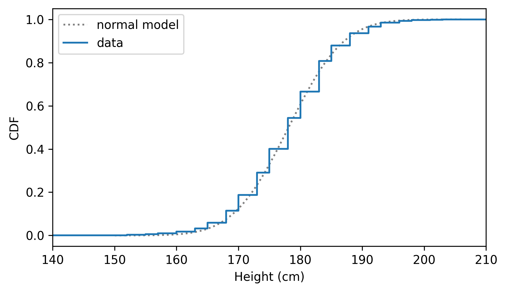
And here’s how it compares to the CDF of the data.

cdf_height = Cdf.from_seq(heights, name="data")
cdf_normal_model.plot(color="gray")
cdf_height.step()

xlim = [140, 210]
decorate(xlabel="Height (cm)", ylabel="CDF", xlim=xlim)

Use gaussian_kde to make an Pdf to represent the PDF of male height. Hint: Investigate the bw_method argument, which can be used to control the smoothness of the estimated density. Plot the estimated density and compare it to a NormalPdf with mean m and standard deviation s.

Use a NormalPdf and area_under to compute the fraction of people in the normal model that are between 178 and 185 centimeters. Use a NormalCdf to compute the same fraction, and check that the results are consistent. Finally, use the empirical Cdf of the data to see what fraction of people in the dataset are in the same range.

Think Stats: Exploratory Data Analysis in Python, 3rd Edition

Copyright 2024 Allen B. Downey

Code license: MIT License

Text license: Creative Commons Attribution-NonCommercial-ShareAlike 4.0 International