The third edition of Think Stats is available now from Bookshop.org and Amazon (those are affiliate links). If you are enjoying the free, online version, consider buying me a coffee.
4. Cumulative Distribution Functions#
Frequency tables and PMFs are the most familiar ways to represent distributions, but as we’ll see in this chapter, they have limitations. An alternative is the cumulative distribution function (CDF), which is useful for computing percentiles, and especially useful for comparing distributions.
Also in this chapter, we’ll compute percentile-based statistics to quantify the location, spread, and skewness of a distribution.
Click here to run this notebook on Colab.
Show code cell content
from os.path import basename, exists


def download(url):
    filename = basename(url)
    if not exists(filename):
        from urllib.request import urlretrieve

        local, _ = urlretrieve(url, filename)
        print("Downloaded " + local)


download("https://github.com/AllenDowney/ThinkStats/raw/v3/nb/thinkstats.py")
Show code cell content
try:
    import empiricaldist
except ImportError:
    %pip install empiricaldist
Show code cell content
import numpy as np
import pandas as pd
import matplotlib.pyplot as plt

from thinkstats import decorate
4.1. Percentiles and Percentile Ranks#
If you have taken a standardized test, you probably got your results in the form of a raw score and a percentile rank. In this context, the percentile rank is the percentage of people who got the same score as you or lower. So if you are “in the 90th percentile,” you did as well as or better than 90% of the people who took the exam.
To understand percentiles and percentile ranks, let’s consider an example based on running speeds. Some years ago I ran the James Joyce Ramble, which is a 10 kilometer road race in Massachusetts. After the race, I downloaded the results to see how my time compared to other runners.
Instructions for downloading the data are in the notebook for this chapter.
download("https://github.com/AllenDowney/ThinkStats/raw/v3/nb/relay.py")
download(
    "https://github.com/AllenDowney/ThinkStats/raw/v3/data/Apr25_27thAn_set1.shtml"
)
The relay.py module provides a function that reads the results and returns a Pandas DataFrame.
from relay import read_results

results = read_results()
results.head()
| Place | Div/Tot | Division | Guntime | Nettime | Min/Mile | MPH | |
|---|---|---|---|---|---|---|---|
| 0 | 1 | 1/362 | M2039 | 30:43 | 30:42 | 4:57 | 12.121212 |
| 1 | 2 | 2/362 | M2039 | 31:36 | 31:36 | 5:06 | 11.764706 |
| 2 | 3 | 3/362 | M2039 | 31:42 | 31:42 | 5:07 | 11.726384 |
| 3 | 4 | 4/362 | M2039 | 32:28 | 32:27 | 5:14 | 11.464968 |
| 4 | 5 | 5/362 | M2039 | 32:52 | 32:52 | 5:18 | 11.320755 |
results contains one row for each of 1633 runners who finished the race.
The column we’ll use to quantify performance is MPH, which contains each runner’s average speed in miles per hour.
We’ll select this column and use values to extract the speeds as a NumPy array.
speeds = results["MPH"].values
I finished in 42:44, so we can find my row like this.
my_result = results.query("Nettime == '42:44'")
my_result
| Place | Div/Tot | Division | Guntime | Nettime | Min/Mile | MPH | |
|---|---|---|---|---|---|---|---|
| 96 | 97 | 26/256 | M4049 | 42:48 | 42:44 | 6:53 | 8.716707 |
The index of my row is 96, so we can extract my speed like this.
my_speed = speeds[96]
We can use sum to count the number of runners at my speed or slower.
(speeds <= my_speed).sum()
np.int64(1537)
And we can use mean to compute the percentage of runners at my speed or slower.
(speeds <= my_speed).mean() * 100
np.float64(94.12124923453766)
The result is my percentile rank in the field, which was about 94%.
More generally, the following function computes the percentile rank of a particular value in a sequence of values.
def percentile_rank(x, seq):
    """Percentile rank of x.

    x: value
    seq: sequence of values

    returns: percentile rank 0-100
    """
    return (seq <= x).mean() * 100
In results, the Division column indicates the division each runner was in, identified by gender and age range – for example, I was in the M4049 division, which includes male runners aged 40 to 49.
We can use the query method to select the rows for people in my division and extract their speeds.
my_division = results.query("Division == 'M4049'")
my_division_speeds = my_division["MPH"].values
Now we can use percentile_rank to compute my percentile rank in my division.
percentile_rank(my_speed, my_division_speeds)
np.float64(90.234375)
Going in the other direction, if we are given a percentile rank, the following function finds the corresponding value in a sequence.
def percentile(p, seq):
    n = len(seq)
    i = (1 - p / 100) * (n + 1)
    return seq[round(i)]
n is the number of elements in the sequence; i is the index of the element with the given percentile rank.
When we look up a percentile rank, the corresponding value is called a percentile.
percentile(90, my_division_speeds)
np.float64(8.591885441527447)
In my division, the 90th percentile was about 8.6 mph.
Now, some years after I ran that race, I am in the M5059 division.
So let’s see how fast I would have to run to have the same percentile rank in my new division.
We can answer that question by converting my percentile rank in the M4049 division, which is about 90.2%, to a speed in the M5059 division.
next_division = results.query("Division == 'M5059'")
next_division_speeds = next_division["MPH"].values

percentile(90.2, next_division_speeds)
np.float64(8.017817371937639)
The person in the M5059 division with the same percentile rank as me ran just over 8 mph.
We can use query to find him.
next_division.query("MPH > 8.01").tail(1)
| Place | Div/Tot | Division | Guntime | Nettime | Min/Mile | MPH | |
|---|---|---|---|---|---|---|---|
| 222 | 223 | 18/171 | M5059 | 46:30 | 46:25 | 7:29 | 8.017817 |
He finished in 46:25 and came in 18th out of 171 people in his division.
With this introduction to percentile ranks and percentiles, we are ready for cumulative distribution functions.
4.2. CDFs#
A cumulative distribution function, or CDF, is another way to describe the distribution of a set of values, along with a frequency table or PMF.
Given a value x, the CDF computes the fraction of values less than or equal to x.
As an example, we’ll start with a short sequence.
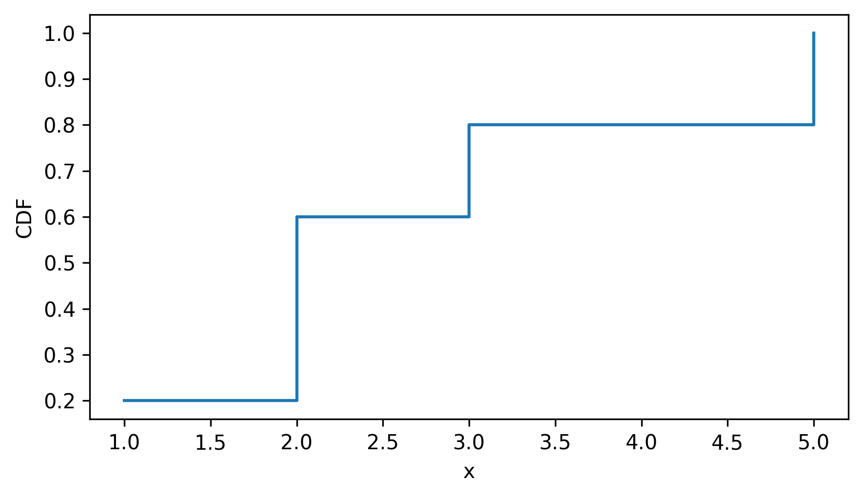
t = [1, 2, 2, 3, 5]
One way to compute a CDF is to start with a PMF.
Here is a Pmf object that represents the distribution of values in t.
from empiricaldist import Pmf

pmf = Pmf.from_seq(t)
pmf
| probs | |
|---|---|
| 1 | 0.2 |
| 2 | 0.4 |
| 3 | 0.2 |
| 5 | 0.2 |
As we saw in the previous chapter, we can use the bracket operator to look up a value in a Pmf.
pmf[2]
np.float64(0.4)
The result is the proportion of values in the sequence equal to the given value.
In this example, two out of five values are equal to 2, so the result is 0.4.
We can also think of this proportion as the probability that a randomly chosen value from the sequence equals 2.
Pmf has a make_cdf method that computes the cumulative sum of the probabilities in the Pmf.
cdf = pmf.make_cdf()
cdf
| probs | |
|---|---|
| 1 | 0.2 |
| 2 | 0.6 |
| 3 | 0.8 |
| 5 | 1.0 |
The result is a Cdf object, which is a kind of Pandas Series.
We can use the bracket operator to look up a value.
cdf[2]
np.float64(0.6000000000000001)
The result is the proportion of values in the sequence less than or equal to the given value. In this example, three out of five values in the sequence are less than or equal to 2, so the result is 0.6.
We can also think of this proportion as the probability that a randomly chosen value from the sequence is less than or equal to 2.
We can use parentheses to call the Cdf object like a function.
cdf(3)
array(0.8)
The cumulative distribution function is defined for all numbers, not just the ones that appear in the sequence.
cdf(4)
array(0.8)
To visualize the Cdf, we can use the step method, which plots the Cdf as a step function.
cdf.step()
decorate(xlabel="x", ylabel="CDF")
As a second example, let’s make a Cdf that represents the distribution of running speeds from the previous section.
The Cdf class provides a from_seq function we can use to create a Cdf object from a sequence.
from empiricaldist import Cdf

cdf_speeds = Cdf.from_seq(speeds)
And here’s what it looks like – the vertical line is at my speed.
cdf_speeds.step()
plt.axvline(my_speed, ls=":", color="gray")
decorate(xlabel="Speed (mph)", ylabel="CDF")
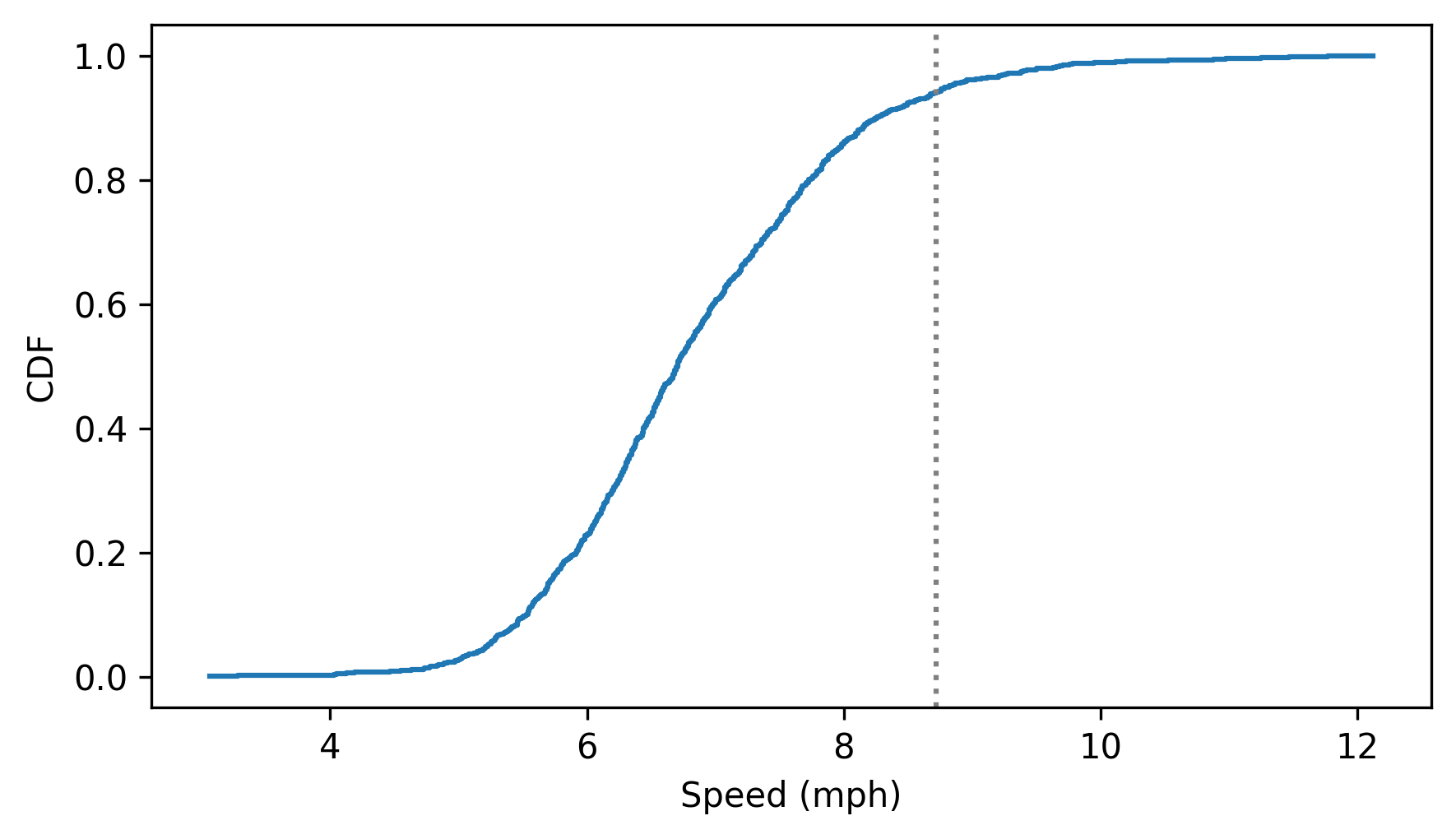
If we look up my speed, the result is the fraction of runners at my speed or slower. If we multiply by 100, we get my percentile rank.
cdf_speeds(my_speed) * 100
np.float64(94.12124923453766)
So that’s one way to think about the Cdf – given a value, it computes something like a percentile rank, except that it’s a proportion between 0 and 1 rather than a percentage between 0 and 100.
Cdf provides an inverse method that computes the inverse of the cumulative distribution function – given a proportion between 0 and 1, it finds the corresponding value.
For example, if someone says they ran as fast or faster than 50% of the field, we can find their speed like this.
cdf_speeds.inverse(0.5)
array(6.70391061)
If you have a proportion and you use the inverse CDF to find the corresponding value, the result is called a quantile – so the inverse CDF is sometimes called the quantile function.
If you have have a quantile and you use the CDF to find the corresponding proportion, the result doesn’t really have a name, strangely. To be consistent with percentile and percentile rank, it could be called a “quantile rank”, but as far as I can tell, no one calls it that. Most often, it is just called a “cumulative probability”.
4.3. Comparing CDFs#
CDFs are especially useful for comparing distributions.
As an example, let’s compare the distribution of birth weights for first babies and others.
We’ll load the NSFG dataset again, and divide it into three DataFrames: all live births, first babies, and others.
The following cells download the data files and install statadict, which we need to read the data.
download("https://github.com/AllenDowney/ThinkStats/raw/v3/nb/nsfg.py")
download("https://github.com/AllenDowney/ThinkStats/raw/v3/data/2002FemPreg.dct")
download("https://github.com/AllenDowney/ThinkStats/raw/v3/data/2002FemPreg.dat.gz")
try:
    import statadict
except ImportError:
    %pip install statadict
from nsfg import get_nsfg_groups

live, firsts, others = get_nsfg_groups()
From firsts and others we’ll select total birth weights in pounds, using dropna to remove values that are nan.
first_weights = firsts["totalwgt_lb"].dropna()
first_weights.mean()
np.float64(7.201094430437772)
other_weights = others["totalwgt_lb"].dropna()
other_weights.mean()
np.float64(7.325855614973262)
It looks like first babies are a little lighter on average. But there are several ways a difference like that could happen – for example, there might be a small number of first babies who are especially light, or a small number of other babies who are especially heavy. In those cases, the distributions would have different shapes. As another possibility, the distributions might have the same shape, but different locations.
To compare the distributions, we can try plotting the PMFs.
from empiricaldist import Pmf

first_pmf = Pmf.from_seq(first_weights, name="first")
other_pmf = Pmf.from_seq(other_weights, name="other")
But as we can see in the following figure, it doesn’t work very well.
from thinkstats import two_bar_plots

two_bar_plots(first_pmf, other_pmf, width=0.06)
decorate(xlabel="Weight (pounds)", ylabel="PMF")
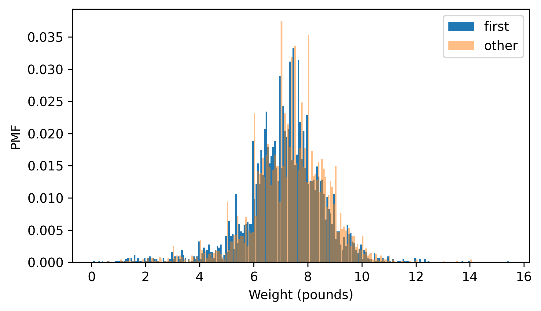
I adjusted the width and transparency of the bars to show the distributions as clearly as possible, but it is hard to compare them. There are many peaks and valleys, and some apparent differences, but it is hard to tell which of these features are meaningful. Also, it is hard to see overall patterns; for example, it is not visually apparent which distribution has the higher mean.
These problems can be mitigated by binning the data – that is, dividing the range of quantities into non-overlapping intervals and counting the number of quantities in each bin. Binning can be useful, but it is tricky to get the size of the bins right. If they are big enough to smooth out noise, they might also smooth out useful information.
A good alternative is to plot the CDFs.
first_cdf = first_pmf.make_cdf()
other_cdf = other_pmf.make_cdf()
Here’s what they look like.
first_cdf.plot(ls="--")
other_cdf.plot(alpha=0.5)
decorate(xlabel="Weight (pounds)", ylabel="CDF")
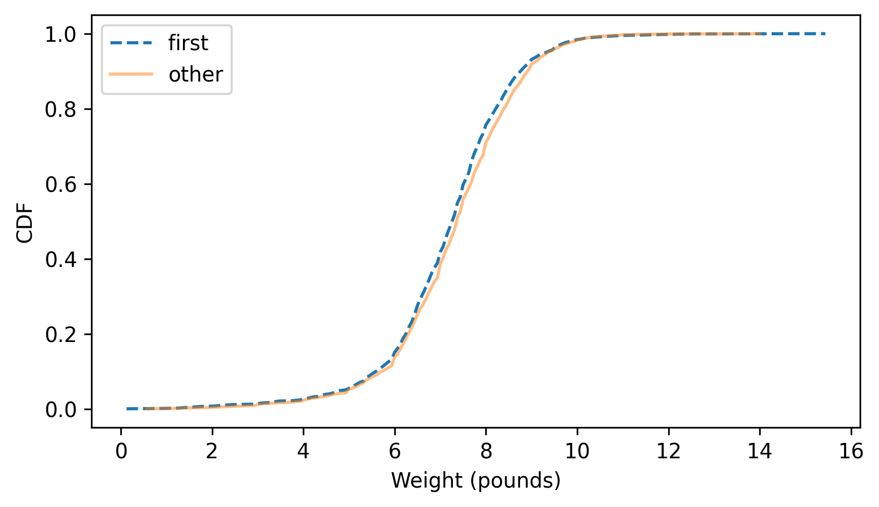
This figure makes the shape of the distributions, and the differences between them, much clearer. The curve for first babies is consistently to the left of the curve for others, which indicates that first babies are slightly lighter throughout the distribution – with a larger discrepancy above the midpoint.
4.4. Percentile-Based Statistics#
In Chapter 3 we computed the arithmetic mean, which identifies a central point in a distribution, and the standard deviation, which quantifies how spread out the distribution is. And in a previous exercise we computed skewness, which indicates whether a distribution is skewed left or right. One drawback of all of these statistics is that they are sensitive to outliers. A single extreme value in a dataset can have a large effect on mean, standard deviation, and skewness.
An alternative is to use statistics that are based on percentiles of the distribution, which tend to be more robust, which means that they are less sensitive to outliers. To demonstrate, let’s load the NSFG data again without doing any data cleaning.
from nsfg import read_stata

dct_file = "2002FemPreg.dct"
dat_file = "2002FemPreg.dat.gz"

preg = read_stata(dct_file, dat_file)
Recall that birth weight is recorded in two columns, one for the pounds and one for the ounces.
birthwgt_lb = preg["birthwgt_lb"]
birthwgt_oz = preg["birthwgt_oz"]
If we make a Hist object with the values from birthwgt_oz, we can see that they include the special values 97, 98, and 99, which indicate missing data.
from empiricaldist import Hist

Hist.from_seq(birthwgt_oz).tail(5)
| freqs | |
|---|---|
| birthwgt_oz | |
| 14.0 | 475 |
| 15.0 | 378 |
| 97.0 | 1 |
| 98.0 | 1 |
| 99.0 | 46 |
The birthwgt_lb column includes the same special values; it also includes the value 51, which has to be a mistake.
Hist.from_seq(birthwgt_lb).tail(5)
| freqs | |
|---|---|
| birthwgt_lb | |
| 15.0 | 1 |
| 51.0 | 1 |
| 97.0 | 1 |
| 98.0 | 1 |
| 99.0 | 57 |
Now let’s imagine two scenarios.
In one scenario, we clean these variables by replacing missing and invalid values with nan, and then compute total weight in pounds.
Dividing birthwgt_oz_clean by 16 converts it to pounds in decimal.
birthwgt_lb_clean = birthwgt_lb.replace([51, 97, 98, 99], np.nan)
birthwgt_oz_clean = birthwgt_oz.replace([97, 98, 99], np.nan)

total_weight_clean = birthwgt_lb_clean + birthwgt_oz_clean / 16
In the other scenario, we neglect to clean the data and accidentally compute the total weight with these bogus values.
total_weight_bogus = birthwgt_lb + birthwgt_oz / 16
The bogus dataset contains only 49 bogus values, which is about 0.5% of the data.
count1, count2 = total_weight_bogus.count(), total_weight_clean.count()
diff = count1 - count2

diff, diff / count2 * 100
(np.int64(49), np.float64(0.5421553441026776))
Now let’s compute the mean of the data in both scenarios.
mean1, mean2 = total_weight_bogus.mean(), total_weight_clean.mean()
mean1, mean2
(np.float64(7.319680587652691), np.float64(7.265628457623368))
The bogus values have a moderate effect on the mean. If we take the mean of the cleaned data to be correct, the mean of the bogus data is off by less than 1%.
(mean1 - mean2) / mean2 * 100
np.float64(0.74394294099376)
An error like that might go undetected – but now let’s see what happens to the standard deviations.
std1, std2 = total_weight_bogus.std(), total_weight_clean.std()
std1, std2
(np.float64(2.096001779161835), np.float64(1.4082934455690173))
(std1 - std2) / std2 * 100
np.float64(48.83274403900607)
The standard deviation of the bogus data is off by almost 50%, so that’s more noticeable. Finally, here’s the skewness of the two datasets.
def skewness(seq):
    """Compute the skewness of a sequence

    seq: sequence of numbers

    returns: float skewness
    """
    deviations = seq - seq.mean()
    return np.mean(deviations**3) / seq.std(ddof=0) ** 3
skew1, skew2 = skewness(total_weight_bogus), skewness(total_weight_clean)
skew1, skew2
(np.float64(22.251846195422484), np.float64(-0.5895062687577697))
# how much is skew1 off by?
(skew1 - skew2) / skew2
np.float64(-38.74658112171128)
The skewness of the bogus dataset is off by a factor of almost 40, and it has the wrong sign! With the outliers added to the data, the distribution is strongly skewed to the right, as indicated by large positive skewness. But the distribution of the valid data is slightly skewed to the left, as indicated by small negative skewness.
These results show that a small number of outliers have a moderate effect on the mean, a strong effect on the standard deviation, and a disastrous effect on skewness.
An alternative is to use statistics based on percentiles. Specifically:
The median, which is the 50th percentile, identifies a central point in a distribution, like the mean.
The interquartile range, which is the difference between the 25th and 75th percentiles, quantifies the spread of the distribution, like the standard deviation.
The quartile skewness uses the quartiles of the distribution (25th, 50th, and 75th percentiles) to quantify the skewness.
The Cdf object provides an efficient way to compute these percentile-based statistics.
To demonstrate, let’s make a Cdf object from the bogus and clean datasets.
cdf_total_weight_bogus = Cdf.from_seq(total_weight_bogus)
cdf_total_weight_clean = Cdf.from_seq(total_weight_clean)
The following function takes a Cdf and uses its inverse method to compute the 50th percentile, which is the median (at least, it is one way to define the median of a dataset).
def median(cdf):
    m = cdf.inverse(0.5)
    return m
Now we can compute the median of both datasets.
median(cdf_total_weight_bogus), median(cdf_total_weight_clean)
(array(7.375), array(7.375))
The results are identical, so in this case, the outliers have no effect on the median at all. In general, outliers have a smaller effect on the median than on the mean.
The interquartile range (IQR) is the difference between the 75th and 25th percentiles.
The following function takes a Cdf and returns the IQR.
def iqr(cdf):
    low, high = cdf.inverse([0.25, 0.75])
    return high - low
And here are the interquartile ranges of the two datasets.
iqr(cdf_total_weight_bogus), iqr(cdf_total_weight_clean)
(np.float64(1.625), np.float64(1.625))
In general, outliers have less effect on the IQR than on the standard deviation – in this case they have no effect at all.
Finally, here’s a function that computes quartile skewness, which depends on three statistics:
The median,
The midpoint of 25th and 75th percentiles, and
The semi-IQR, which is half of the IQR.
def quartile_skewness(cdf):
    low, median, high = cdf.inverse([0.25, 0.5, 0.75])
    midpoint = (high + low) / 2
    semi_iqr = (high - low) / 2
    return (midpoint - median) / semi_iqr
And here’s the quartile skewness for the two datasets.
qskew1 = quartile_skewness(cdf_total_weight_bogus)
qskew2 = quartile_skewness(cdf_total_weight_clean)
qskew1, qskew2
(np.float64(-0.07692307692307693), np.float64(-0.07692307692307693))
The small number of outliers in these examples has no effect on the quartile skewness. These examples show that percentile-based statistics are less sensitive to outliers and errors in the data.
4.5. Random Numbers#
Cdf objects provide an efficient way to generate random numbers from a distribution.
First we generate random numbers from a uniform distribution between 0 and 1.
Then we evaluate the inverse CDF at those points.
The following function implements this algorithm.
def sample_from_cdf(cdf, n):
    ps = np.random.random(size=n)
    return cdf.inverse(ps)
To demonstrate, let’s generate a random sample of running speeds.
sample = sample_from_cdf(cdf_speeds, 1001)
To confirm that it worked, we can compare the CDFs of the sample and the original dataset.
cdf_sample = Cdf.from_seq(sample)

cdf_speeds.plot(label="original", ls="--")
cdf_sample.plot(label="sample", alpha=0.5)

decorate(xlabel="Speed (mph)", ylabel="CDF")
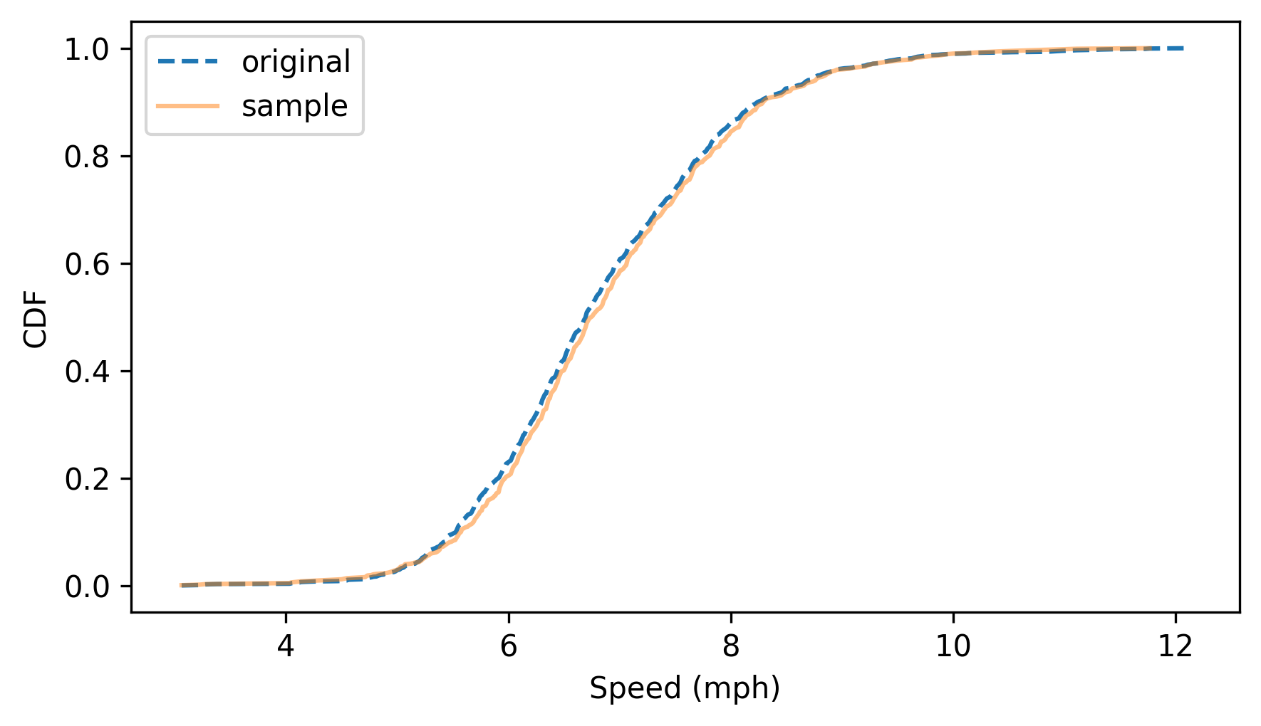
The sample follows the distribution of the original data. To understand how this algorithm works, consider this question: Suppose we choose a random sample from the population of running speeds and look up the percentile ranks of the speeds in the sample. Now suppose we compute the CDF of the percentile ranks. What do you think it will look like?
Let’s find out. Here are the percentile ranks for the sample we generated.
percentile_ranks = cdf_speeds(sample) * 100
And here is the CDF of the percentile ranks.
cdf_percentile_rank = Cdf.from_seq(percentile_ranks)
cdf_percentile_rank.plot()

decorate(xlabel="Percentile rank", ylabel="CDF")
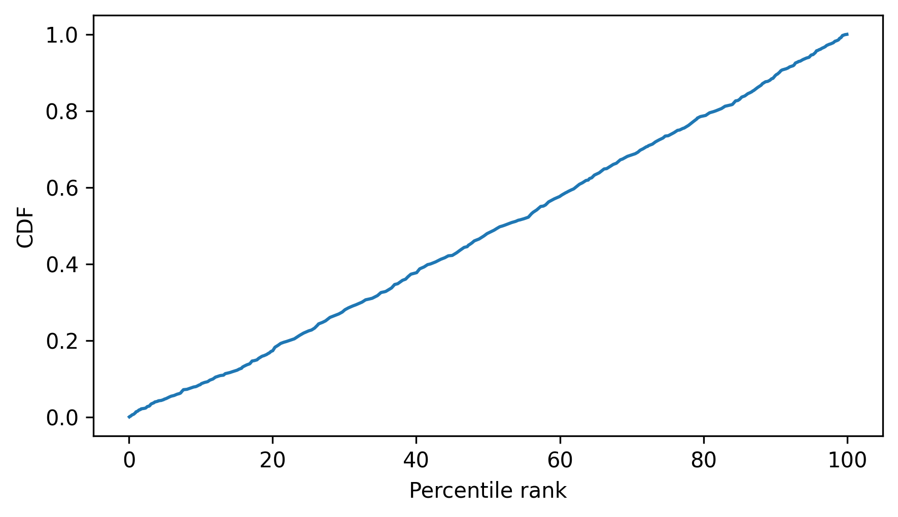
The CDF of the percentile ranks is close to a straight line between 0 and 1. And that makes sense, because in any distribution, the proportion with percentile rank less than 50% is 0.5; the proportion with percentile rank less than 90% is 0.9, and so on.
Cdf provides a sample method that uses this algorithm, so we could also generate a sample like this.
sample = cdf_speeds.sample(1001)
4.6. Glossary#
percentile rank: The percentage of values in a distribution that are less than or equal to a given quantity.
percentile: The value in a distribution associated with a given percentile rank.
cumulative distribution function (CDF): A function that maps a value to the proportion of the distribution less than or equal to that value.
quantile: The value in a distribution that is greater than or equal to a given proportion of values.
robust: A statistic is robust if it is less affected by extreme values or outliers.
interquartile range (IQR): The difference between the 75th and 25th percentiles, used to measure the spread of a distribution.
4.7. Exercises#
4.7.1. Exercise 4.1#
How much did you weigh at birth? If you don’t know, call your mother or someone else who knows. And if no one knows, you can use my birth weight, 8.5 pounds, for this exercise.
Using the NSFG data (all live births), compute the distribution of birth weights and use it to find your percentile rank. If you were a first baby, find your percentile rank in the distribution for first babies. Otherwise use the distribution for others. If you are in the 90th percentile or higher, call your mother back and apologize.
from nsfg import get_nsfg_groups

live, firsts, others = get_nsfg_groups()
4.7.2. Exercise 4.2#
For live births in the NSFG dataset, the column babysex indicates whether the baby was male or female.
We can use query to select the rows for male and female babies.
male = live.query("babysex == 1")
female = live.query("babysex == 2")
len(male), len(female)
(4641, 4500)
Make Cdf objects that represent the distribution of birth weights for male and female babies.
Plot the two CDFs.
What are the differences in the shape and location of the distributions?
If a male baby weighs 8.5 pounds, what is his percentile rank? What is the weight of a female baby with the same percentile rank?
4.7.3. Exercise 4.3#
From the NSFG dataset pregnancy data, select the agepreg column and make a Cdf to represent the distribution of age at conception for each pregnancy.
Use the CDF to compute the percentage of ages less than or equal to 20, and the percentage less than or equal to 30.
Use those results to compute the percentage between 20 and 30.
from nsfg import read_fem_preg

preg = read_fem_preg()
4.7.4. Exercise 4.4#
Here are the running speeds of the people who finished the James Joyce Ramble, described earlier in this chapter.
speeds = results["MPH"].values
Make a Cdf that represents the distribution of these speeds, and use it to compute the median, IQR, and quartile skewness.
Does the distribution skew to the left or right?
4.7.5. Exercise 4.5#
The numbers generated by np.random.random are supposed to be uniform between 0 and 1, which means that the CDF of a sample should be a straight line.
Let’s see if that’s true.
Here’s a sample of 1001 numbers. Plot the CDF of this sample. Does it look like a straight line?
t = np.random.random(1001)
Think Stats: Exploratory Data Analysis in Python, 3rd Edition
Copyright 2024 Allen B. Downey
Code license: MIT License
Text license: Creative Commons Attribution-NonCommercial-ShareAlike 4.0 International