Introduction
In most countries, women live longer than men. This difference is often assumed to be natural and inevitable -- and sometimes desirable. For example, in the World Economic Forum’s Global Gender Gap Report, a smaller gap is interpreted as evidence of discrimination against women.
But the gap varies substantially between countries and has changed over time, which suggests that it might not be entirely natural, or if it is, it can be mitigated. For example, in the Netherlands the gap in healthy life expectancy is now close to zero.
The goal of this investigation is to explore differences in life expectancy and health-adjusted life expectancy (HALE) between countries, to identify the factors that contribute to the observed gender gaps, and to estimated the changes needed to close those gaps by improving health outcomes for both men and women.
We use Elastic Net regression to model the gender gap in life expectancy and HALE as a function of cause-specific mortality indicators. This approach handles the high correlation among predictors and identifies patterns of mortality most strongly associated with the life expectancy gap.
Data
The analysis uses data from two sources:
WHO Global Health Observatory (GHO) API: Provides HALE and life expectancy. Data is accessed programmatically via the GHO OData API.
IHME Global Burden of Disease: Provides most cause-specific mortality indicators with better temporal coverage than WHO, including cardiovascular disease, diabetes, chronic respiratory disease, neoplasms (cancer), alcohol use disorders, self-harm (suicide), interpersonal violence (homicide), road injuries, unintentional injuries, liver disease, and drug use disorders.
For each indicator, we use the most recent available data from 2000-2019. We exclude 2020 and later years to avoid distortions from the COVID-19 pandemic, which had significant impacts on mortality patterns that may not reflect underlying health factors. Using 2019 or earlier data provides a more stable baseline for understanding the gender gap.
The analysis focuses on OECD countries (38 countries) to ensure consistent data quality and comparability. For each country, we compute gender gaps by taking the difference between female and male values for each indicator.
Early-life mortality indicators (infant and under-five mortality) were considered but excluded from the final model because they had very low importance and limited temporal coverage. The IHME alternative (all-cause deaths under 5, per 100,000 population) was also considered but excluded because it is confounded with age structure and fertility rates, making it methodologically inappropriate for cross-country comparison.
Target Variables
The analysis focuses on two target variables:
HALE Gap: The difference in Healthy Life Expectancy between women and men (Female - Male, in years)
Life Expectancy Gap: The difference in Life Expectancy between women and men (Female - Male, in years)
The following table shows the median, minimum, and maximum values for HALE and Life Expectancy across OECD countries.
| Indicator | Median | Min | Max |
|---|---|---|---|
| HALE | 70.1 | 65.5 | 73.5 |
| Life Expectancy | 81.4 | 75.5 | 84.4 |
The following table shows the median, minimum, and maximum gender gaps (Female - Male) for HALE and Life Expectancy across OECD countries.
| Indicator | Median Gap | Min Gap | Max Gap |
|---|---|---|---|
| HALE | 1.39 | 0.0186 | 6.06 |
| Life Expectancy | 4.56 | 2.8 | 9.36 |
The following table shows the HALE and Life Expectancy gaps for all OECD countries, sorted by HALE gap:
| Country | HALE_Gap | LifeExpectancy_Gap |
|---|---|---|
| Lithuania | 6.06 | 9.36 |
| Latvia | 5.69 | 8.92 |
| Poland | 4.93 | 7.92 |
| Estonia | 4.79 | 7.55 |
| Slovakia | 3.93 | 6.67 |
| Hungary | 3.72 | 6.54 |
| South Korea | 3.56 | 6.09 |
| Mexico | 3.1 | 6.01 |
| Czechia | 3.09 | 5.77 |
| Japan | 2.93 | 5.63 |
| Slovenia | 2.91 | 5.47 |
| Colombia | 2.89 | 5.45 |
| Portugal | 2.39 | 5.38 |
| Costa Rica | 2.26 | 5.22 |
| Finland | 2.24 | 5.12 |
| France | 1.82 | 5.04 |
| United States | 1.8 | 5.04 |
| Spain | 1.52 | 4.78 |
| Chile | 1.41 | 4.68 |
| Austria | 1.36 | 4.45 |
| Greece | 1.33 | 4.44 |
| Canada | 1.25 | 4.33 |
| Türkiye | 1.17 | 4.21 |
| Australia | 1.16 | 4.15 |
| Italy | 1.07 | 3.98 |
| Belgium | 0.941 | 3.92 |
| Luxembourg | 0.915 | 3.85 |
| Denmark | 0.895 | 3.77 |
| Germany | 0.862 | 3.58 |
| United Kingdom | 0.695 | 3.57 |
| Israel | 0.611 | 3.42 |
| New Zealand | 0.487 | 3.36 |
| Ireland | 0.454 | 3.33 |
| Switzerland | 0.338 | 3.27 |
| Norway | 0.239 | 3.07 |
| Iceland | 0.16 | 3.04 |
| Sweden | 0.134 | 2.91 |
| Netherlands | 0.0186 | 2.8 |
In several countries, mostly in Northern Europe, the HALE gap is effectively zero, and the gap in life expectancy is three years or less. These countries are evidence that there is nothing inevitable about these gaps, and no unavoidable reason for gaps as high as 5 years in the United States or 9 years in Latvia and Lithuania.
Predictors
The following tables summarize the predictors used to explain variation in the HALE and Life Expectancy gender gaps. Each predictor includes:
Median Rate: The median across countries of the overall rate (computed as the average of male and female rates)
Min Rate / Max Rate: The range of overall rates across countries
Median Gap: The median gender gap (Male - Female for predictors) across countries
Min Gap / Max Gap: The range of gender gaps across countries
Corr HALE: Correlation with HALE gap
Corr LE: Correlation with Life Expectancy gap
For each predictor, the following table shows overall rates in deaths per 100,000 people (computed as the average of male and female rates).
| Indicator | Median Rate | Min Rate | Max Rate | Corr HALE | Corr LE |
|---|---|---|---|---|---|
| Neoplasms | 265 | 80.3 | 365 | 0.214 | 0.228 |
| Cardiovascular | 241 | 113 | 746 | 0.689 | 0.721 |
| ChronicRespiratory | 43.7 | 17.1 | 85.4 | -0.537 | -0.517 |
| UnintentionalInjury | 26.5 | 10.7 | 46.4 | 0.22 | 0.259 |
| Diabetes | 18.5 | 7.4 | 61 | 0.338 | 0.377 |
| LiverDisease | 15.5 | 3.09 | 36.5 | 0.734 | 0.74 |
| Suicide | 13 | 4.2 | 29.5 | 0.538 | 0.511 |
| RoadTraffic | 5.68 | 2.46 | 16.2 | 0.445 | 0.418 |
| Alcohol | 3.09 | 0.193 | 15 | 0.559 | 0.545 |
| DrugDisorder | 2.14 | 0.212 | 20.8 | -0.194 | -0.232 |
| Homicide | 1.13 | 0.457 | 30.5 | 0.256 | 0.213 |
The highest death rates are from cancer (neoplasms) and cardiovascular disease, followed by chronic respiratory disease. Death rates due to alcohol use disorders are much smaller than the highest rates, but as we’ll see, cancer-related deaths and other factors are the primary contributors to gender gaps in life expectancy.
Several predictors are strongly correlated with life expectancy gaps, notably Neoplasms and Unintentional Injury. Most of the correlations are positive, indicating that countries with higher death rates also have larger gender gaps.
The following table shows gender gaps (Male - Female) in death rates for each predictor.
| Indicator | Median Gap | Min Gap | Max Gap | Corr HALE | Corr LE |
|---|---|---|---|---|---|
| Neoplasms | 57.6 | -0.788 | 132 | 0.454 | 0.519 |
| Suicide | 13.8 | 4.51 | 40.2 | 0.748 | 0.733 |
| LiverDisease | 9.65 | 1.29 | 32.6 | 0.724 | 0.733 |
| ChronicRespiratory | 8.03 | -19.3 | 34.1 | 0.475 | 0.55 |
| RoadTraffic | 5.6 | 2.04 | 22 | 0.42 | 0.402 |
| UnintentionalInjury | 4.95 | -11.2 | 37.1 | 0.833 | 0.848 |
| Alcohol | 3.57 | 0.306 | 23.6 | 0.618 | 0.602 |
| DrugDisorder | 1.66 | 0.0226 | 16 | -0.0636 | -0.0932 |
| Homicide | 0.887 | -0.0622 | 47.5 | 0.233 | 0.19 |
| Diabetes | -0.173 | -9.83 | 5.5 | -0.478 | -0.564 |
| Cardiovascular | -19 | -124 | 25.6 | -0.596 | -0.633 |
Many of the death rates gaps are strongly correlated with life expectancy gaps, which is not surprising -- in a country where more men suffer from alcohol-related disease, for example, we expect a larger gap in both HALE and life expectancy.
Correlations
Many of these predictors are also related to each other. The following table shows the top correlations between the overall rates of different indicators.
| Rate 1 | Rate 2 | Correlation |
|---|---|---|
| UnintentionalInjury | Neoplasms | 0.721 |
| RoadTraffic | Homicide | 0.687 |
| Cardiovascular | Neoplasms | 0.633 |
| Cardiovascular | LiverDisease | 0.631 |
| Alcohol | Cardiovascular | 0.61 |
| Homicide | Neoplasms | -0.601 |
| UnintentionalInjury | Suicide | 0.591 |
| Alcohol | UnintentionalInjury | 0.543 |
| UnintentionalInjury | Cardiovascular | 0.536 |
| Alcohol | Suicide | 0.534 |
The following table shows the top correlations between the gender gaps of different indicators.
| Gap 1 | Gap 2 | Correlation |
|---|---|---|
| ChronicRespiratory | Neoplasms | 0.734 |
| RoadTraffic | Homicide | 0.723 |
| Alcohol | Cardiovascular | -0.688 |
| Alcohol | Suicide | 0.675 |
| UnintentionalInjury | Suicide | 0.633 |
| Cardiovascular | Suicide | -0.613 |
| UnintentionalInjury | LiverDisease | 0.577 |
| Cardiovascular | Neoplasms | -0.564 |
| ChronicRespiratory | Diabetes | -0.564 |
| Alcohol | LiverDisease | 0.542 |
The following table shows the correlation between the overall rate and the gender gap for each predictor. This identifies indicators where countries with higher overall rates also tend to have larger gender gaps.
| Indicator | Correlation |
|---|---|
| Homicide | 0.999 |
| Alcohol | 0.982 |
| RoadTraffic | 0.971 |
| DrugDisorder | 0.957 |
| LiverDisease | 0.955 |
| Suicide | 0.9 |
| Neoplasms | 0.685 |
| UnintentionalInjury | 0.0346 |
| ChronicRespiratory | -0.0787 |
| Diabetes | -0.325 |
| Cardiovascular | -0.804 |
So there are clusters of indicators that move together, both in their overall rates and in their gender gaps.
Methodology
If we put all of these predictors into a single ordinary least squares (OLS) regression, the model is forced to divide the explanatory “credit” among highly correlated variables. In that setting:
Small amounts of noise can change which variable gets the larger coefficient.
Coefficients within a correlated cluster can flip sign or change magnitude dramatically.
The allocation of effect size among correlated predictors is essentially arbitrary.
As a result, an OLS model with all indicators included does not give a stable or interpretable answer to the question “which factors matter most?”.
Elastic Net regression can help. It combines two kinds of regularization:
An L2 (ridge) component that stabilizes coefficients and allows correlated predictors to share weight.
An L1 (lasso) component that shrinks some coefficients all the way to zero when they do not improve predictive performance.
The model is tuned by cross-validation, so the amount of regularization is chosen to maximize out-of-sample predictive accuracy, not to fit the particular noise pattern in the dataset.
In practice, this means:
Correlated predictors are handled coherently, with coefficients shrunk toward each other and toward zero.
Predictors that do not add predictive information beyond the ones already in the model are often assigned coefficients very close to zero.
The remaining non-zero coefficients identify a smaller set of predictors that are genuinely helpful for predicting the life expectancy gap.
That does not mean that every non-zero coefficient in the regression can be interpreted as a causal effect. But it does mean:
Predictors with a stronger direct influence on sex-specific mortality should generally be more predictive of the life expectancy gap.
Predictors that are only loosely or indirectly associated with these mortality differences should contribute less to out-of-sample prediction.
So when Elastic Net assigns substantial weight to a predictor like Alcohol or Neoplasms, we can take that as evidence that these factors are causative, which suggests that efforts to close gaps in these death rates would also close gaps in life expectancy.
Results
Life expectancy gap
We fit three regularized regression models (Ridge, Lasso, and Elastic Net) to predict the Life Expectancy gender gap as a function of cause-specific death rates and gender gaps in those rates. All models use 5-fold cross-validation for model selection and evaluation.
The following table compares the three models using cross-validation R² and mean absolute error:
| Model | CV_R2_Score | CV_MAE_Mean | CV_MAE_Std |
|---|---|---|---|
| Elastic Net | 0.879 | 0.326 | 0.0748 |
| Lasso | 0.878 | 0.337 | 0.0818 |
| Ridge | 0.869 | 0.308 | 0.117 |
Elastic Net performs best with a cross-validation R² of 0.879, meaning it explains about 88% of the variance in the life expectancy gap across OECD countries. The mean absolute error is 0.326 years, indicating that on average, the model’s predictions are off by about 4 months.
Elastic Net selects 13 out of 23 predictors as having non-zero coefficients, effectively performing feature selection while maintaining good predictive performance. The following table shows how many predictors each model uses:
| Model | Total_Predictors | Non_Zero_Coefficients | Zero_Coefficients |
|---|---|---|---|
| Ridge | 22 | 22 | 0 |
| Lasso | 22 | 10 | 12 |
| Elastic Net | 22 | 13 | 9 |
To understand which factors contribute most to the life expectancy gap, we calculate feature importance as the absolute value of the coefficient multiplied by the standard deviation of the predictor. This measures each predictor’s contribution to gap variation on the original scale.
The following figure shows all predictors with non-zero coefficients by importance:
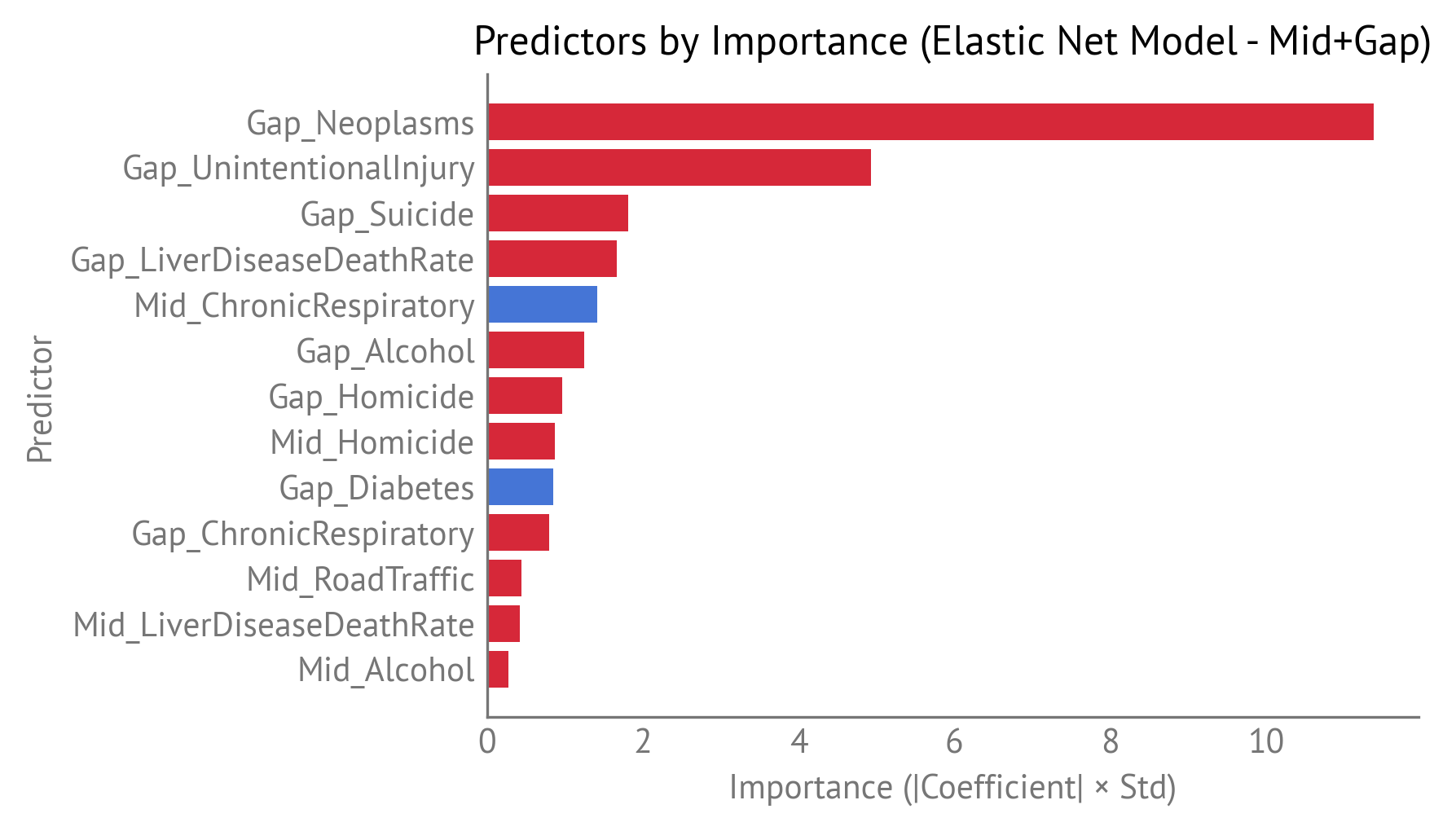
Predictors by importance.
The Neoplasms gap is the most important predictor, with an importance of 11.4. This means that differences in cancer death rates between men and women are the strongest driver of the life expectancy gender gap across OECD countries.
When we aggregate importance by indicator (combining Mid and Gap predictors), we can see which health indicators matter most overall:
| Indicator | Mid_Importance | Gap_Importance | Total_Importance |
|---|---|---|---|
| Neoplasms | 0 | 11.4 | 11.4 |
| UnintentionalInjury | 0 | 4.93 | 4.93 |
| ChronicRespiratory | 1.42 | 0.802 | 2.22 |
| LiverDiseaseDeathRate | 0.418 | 1.67 | 2.08 |
| Homicide | 0.869 | 0.966 | 1.84 |
| Suicide | 0 | 1.82 | 1.82 |
| Alcohol | 0.281 | 1.25 | 1.53 |
| Diabetes | 0 | 0.848 | 0.848 |
| RoadTraffic | 0.442 | 0 | 0.442 |
| Cardiovascular | 0 | 0 | 0 |
| DrugDisorder | 0 | 0 | 0 |
The following figure visualizes indicator-level importance:
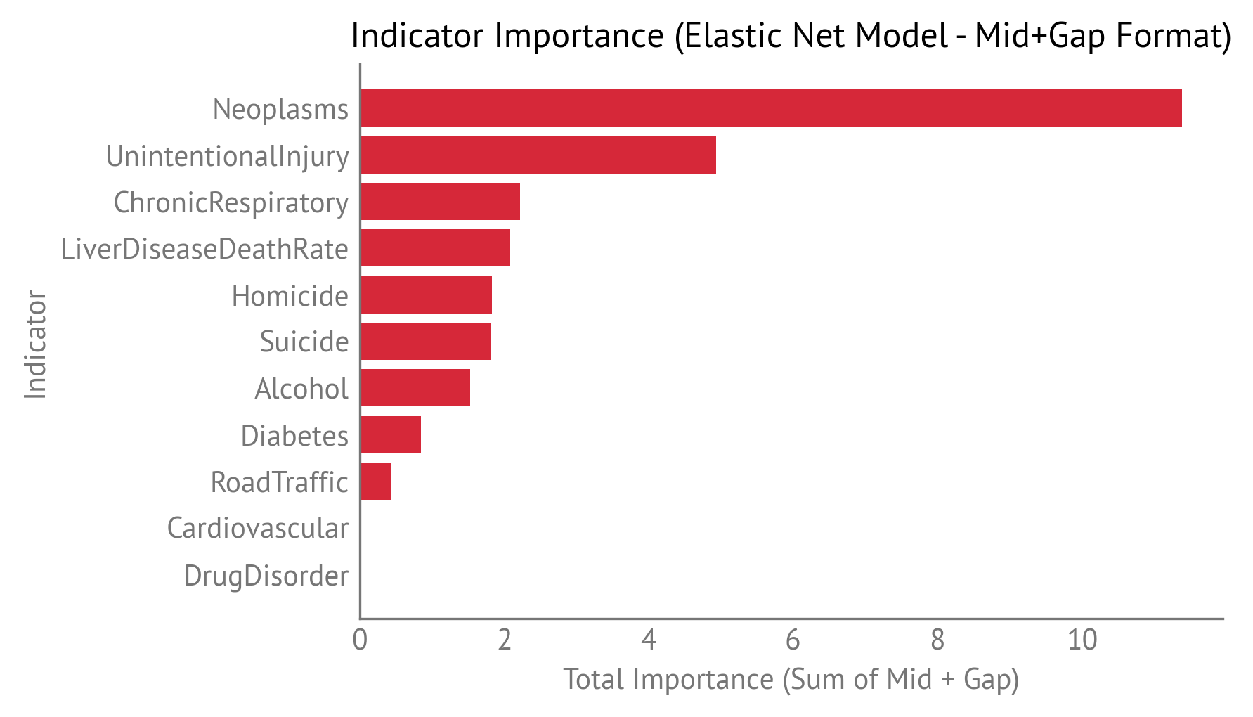
Indicator-level importance, showing which health indicators contribute most to explaining the life expectancy gender gap.
The top indicators are:
Neoplasms (total importance: 11.4) — Cancer death rates are the dominant factor, with importance coming entirely from the gap component, not the overall rate. Some part of this gap is due to past smoking patterns, as men historically smoked more than women. As smoking rates continue to decline, this gap will likely shrink without further intervention, though efforts to reduce smoking should continue.
Unintentional Injury (total importance: 4.93) — Unintentional injuries are the second most important factor, with importance coming entirely from the gap component. These injuries often show gender differences due to occupational exposures, risk-taking behaviors, and activity patterns.
Chronic Respiratory disease (total importance: 2.22) — Chronic respiratory disease contributes moderately, with contributions from both the overall rate and the gender gap. Like neoplasms, some part of the Chronic Respiratory disease gap is due to past smoking patterns, so it will likely shrink as smoking rates continue to decline.
Liver Disease (total importance: 2.08) — Liver disease death rates contribute moderately, with importance coming mostly from the gap component. Liver disease is often related to alcohol consumption, but also includes non-alcoholic causes such as viral hepatitis and non-alcoholic fatty liver disease.
Homicide (total importance: 1.84) — Homicide contributes moderately, with contributions from both the overall rate and the gender gap. Homicide rates are typically much higher in men than women across most countries. Homicide gained substantial importance after removing the childhood mortality indicator, suggesting it may have been capturing some shared variance.
Suicide (total importance: 1.82) — Suicide rates contribute moderately, with importance coming entirely from the gap component. Suicide rates are typically much higher in men than women across most countries.
Alcohol (total importance: 1.53) — Alcohol use disorder death rates contribute moderately, with importance coming mostly from the gap component. The importance is lower than in previous analyses because the current model uses IHME data, which defines alcohol-related mortality more narrowly than WHO’s broader “alcohol-attributable” definition.
Cardiovascular disease has zero importance in this model, meaning it was not selected by Elastic Net as a predictive factor for the life expectancy gap.
Residuals
The following table shows country-level predictions and residuals:
| Country | Actual_HALE_Gap | Predicted_HALE_Gap | Residual | Abs_Residual |
|---|---|---|---|---|
| Sweden | 3.07 | 3.66 | -0.584 | 0.584 |
| France | 5.38 | 4.83 | 0.551 | 0.551 |
| Greece | 4.21 | 4.74 | -0.526 | 0.526 |
| Belgium | 4.15 | 4.66 | -0.511 | 0.511 |
| Austria | 4.33 | 4.8 | -0.47 | 0.47 |
| South Korea | 6.01 | 5.58 | 0.425 | 0.425 |
| Türkiye | 5.04 | 4.64 | 0.396 | 0.396 |
| Costa Rica | 4.78 | 5.17 | -0.386 | 0.386 |
| Latvia | 8.92 | 8.55 | 0.368 | 0.368 |
| Colombia | 5.22 | 4.9 | 0.32 | 0.32 |
| Estonia | 7.92 | 7.61 | 0.313 | 0.313 |
| Finland | 5.04 | 5.33 | -0.286 | 0.286 |
| Spain | 5.12 | 4.85 | 0.273 | 0.273 |
| United States | 4.45 | 4.22 | 0.234 | 0.234 |
| Hungary | 6.54 | 6.31 | 0.234 | 0.234 |
| Germany | 4.44 | 4.64 | -0.208 | 0.208 |
| Chile | 4.68 | 4.88 | -0.203 | 0.203 |
| Poland | 7.55 | 7.37 | 0.188 | 0.188 |
| New Zealand | 3.27 | 3.45 | -0.178 | 0.178 |
| Canada | 3.77 | 3.6 | 0.172 | 0.172 |
| Iceland | 2.8 | 2.96 | -0.158 | 0.158 |
| Slovakia | 6.67 | 6.53 | 0.139 | 0.139 |
| Czechia | 5.63 | 5.76 | -0.127 | 0.127 |
| Netherlands | 2.91 | 3.03 | -0.116 | 0.116 |
| Switzerland | 3.36 | 3.47 | -0.111 | 0.111 |
| Luxembourg | 3.92 | 3.81 | 0.11 | 0.11 |
| Portugal | 5.77 | 5.87 | -0.0978 | 0.0978 |
| Denmark | 3.57 | 3.48 | 0.0952 | 0.0952 |
| United Kingdom | 3.42 | 3.51 | -0.0876 | 0.0876 |
| Mexico | 6.09 | 6.01 | 0.0793 | 0.0793 |
| Australia | 3.85 | 3.78 | 0.0653 | 0.0653 |
| Lithuania | 9.36 | 9.31 | 0.0492 | 0.0492 |
| Ireland | 3.33 | 3.29 | 0.0405 | 0.0405 |
| Israel | 3.58 | 3.54 | 0.0342 | 0.0342 |
| Italy | 3.98 | 4.01 | -0.0334 | 0.0334 |
| Japan | 5.45 | 5.42 | 0.0302 | 0.0302 |
| Slovenia | 5.47 | 5.49 | -0.0195 | 0.0195 |
| Norway | 3.04 | 3.05 | -0.0138 | 0.0138 |
The model shows good fit with residuals distributed around zero across countries.
The model shows good fit with no obvious systematic patterns in the residuals. The following figure shows residuals plotted against predicted values:
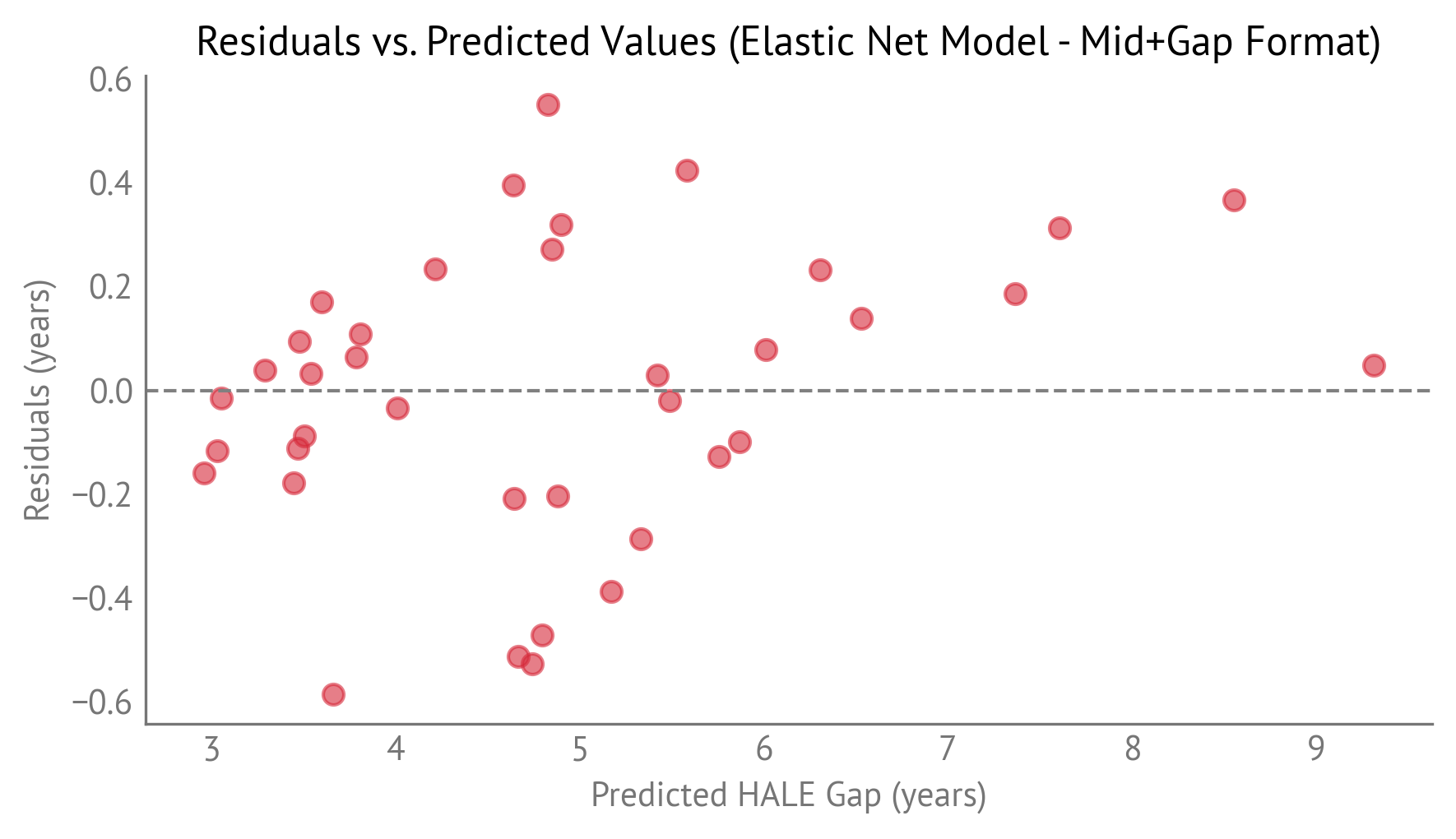
Residuals plotted against predicted life expectancy gap values.
The points are scattered around zero with no obvious patterns, suggesting the model captures the relationship well.
Comparison with Ordinary Least Squares
For comparison, we also fit an ordinary least squares (OLS) model using only the 17 predictors selected by Elastic Net. The following table compares performance:
| Model | R² | Adjusted R² | MAE | Number of Predictors | Non-Zero Coefficients |
|---|---|---|---|---|---|
| Elastic Net | 0.971 | 0.217 | 22 | 13 | |
| OLS (Selected Predictors) | 0.975 | 0.962 | 0.203 | 13 | 13 |
Both models perform similarly, with OLS achieving a slightly higher R² and lower MAE on the training data. However, the cross-validation R² of 0.872 for Elastic Net is a better estimate of out-of-sample performance. The difference between in-sample and cross-validation R² indicates some overfitting, which is expected with a small sample size (38 countries) and many predictors.
Counterfactual Analysis
To understand what it would take to close the life expectancy gender gap, we perform a counterfactual analysis that asks: “What would happen to a country’s predicted life expectancy gap if we adjusted each gap predictor to the best attainable value?”
For each gap predictor, we identify the best attainable value by comparing the current gap to observed gaps in other countries:
If the current gap is positive (Male > Female), we find the country with the smallest gap (most negative).
If the current gap is negative (Female > Male), we find the country with the largest gap (most positive).
If the target gap has the opposite sign of the current gap, we infer that it is possible for the gap to be zero, so we set the target to zero.
To achieve the target gap, we adjust the underlying male or female values:
If the gap is positive (Male > Female), we bring men toward women’s level by reducing the male rate.
If the gap is negative (Female > Male), we bring women toward men’s level by reducing the female rate.
After adjusting the male and female values, we recompute the Mid and Gap values, then use the model to generate a counterfactual prediction. The difference between the original and counterfactual predictions shows how much the life expectancy gap would change if that predictor gap were reduced to the best attainable level (assuming that the relationship is causative).
This approach is conservative in two ways:
We only adjust gap variables, not overall rates, because we’re more confident that gap variables have a causal relationship with the life expectancy gap.
We use other countries as evidence of what’s attainable. If no country has closed or reversed the gap, we assume that the lowest observed gap is the lowest attainable.
The following table shows counterfactual results for the United States.
| Indicator | Current gap | Target gap | Target Country | Change in LE gap |
|---|---|---|---|---|
| Neoplasms | 25.7 | 0 | -0.214 | |
| UnintentionalInjury | 5.26 | 0 | -0.301 | |
| ChronicRespiratory | -5.82 | 0 | 0.0572 | |
| LiverDiseaseDeathRate | 9.05 | 1.29 | Iceland | -0.203 |
| Homicide | 7.29 | 0 | -0.135 | |
| Suicide | 17.3 | 4.51 | Türkiye | -0.537 |
| Alcohol | 5.54 | 0.306 | Colombia | -0.241 |
| Diabetes | 5.5 | 0 | 0.432 | |
| RoadTraffic | 11.2 | 2.04 | Iceland | -0.156 |
| Cardiovascular | 19.4 | 0 | 0 | |
| DrugDisorder | 16 | 0.0226 | Japan | 0 |
The table is sorted by importance, which indicates in general how effective it is to reduce a particular gap. The counterfactual results (the “Change in LE gap” column) indicate how much reducing that gap would specifically affect the life expectancy gap in the United States, which depends on how far the United States is from the target gap for that indicator.
The results show that reducing the Suicide gap from 17.3 to 4.51 (the level observed in Türkiye) would reduce the predicted life expectancy gap by 0.537 years, the largest single impact. Reducing the Unintentional Injury gap to zero would reduce the LE gap by an additional 0.301 years. Reducing the Alcohol gap from 5.54 to 0.306 (the level observed in Colombia) would reduce the gap by 0.241 years. Reducing the Neoplasms gap to zero would reduce the gap by 0.214 years.
Most indicators show negative changes (gap-closing effects), but a few show positive changes (gap-widening effects). The positive changes occur when reducing a gap predictor would increase the life expectancy gap, which can happen when the relationship between predictors and the outcome is complex due to correlations among indicators.
When we sum the effects across all indicators, we can see the total potential impact:
Gap-closing indicators (negative changes): The sum of all indicators that would reduce the life expectancy gap includes Suicide (-0.537), Unintentional Injury (-0.301), Alcohol (-0.241), Neoplasms (-0.214), Liver Disease (-0.203), Road Traffic (-0.156), and Homicide (-0.135), for a total reduction of -1.79 years.
Gap-widening indicators (positive changes): The sum of all indicators that would increase the life expectancy gap includes Diabetes (+0.432) and Chronic Respiratory disease (+0.057), for a total increase of +0.49 years.
The net effect of closing all gaps to their target levels would be a reduction in the predicted life expectancy gap. This represents a substantial part of the current gap.
Healthy Life Expectancy (HALE) Gap
We fit the same three regularized regression models (Ridge, Lasso, and Elastic Net) to predict the HALE gender gap. The following table compares the three models using cross-validation R² and mean absolute error:
| Model | CV_R2_Score | CV_MAE_Mean | CV_MAE_Std |
|---|---|---|---|
| Ridge | 0.79 | 0.396 | 0.105 |
| Elastic Net | 0.778 | 0.422 | 0.119 |
| Lasso | 0.684 | 0.5 | 0.229 |
Elastic Net performs best with a cross-validation R² of 0.778, meaning it explains about 78% of the variance in the HALE gap across OECD countries. The mean absolute error is 0.422 years, indicating that on average, the model’s predictions are off by about 5 months.
The following table shows how many predictors each model uses:
| Model | Total_Predictors | Non_Zero_Coefficients | Zero_Coefficients |
|---|---|---|---|
| Ridge | 22 | 22 | 0 |
| Lasso | 22 | 12 | 10 |
| Elastic Net | 22 | 20 | 2 |
Elastic Net selects 20 out of 22 predictors as having non-zero coefficients. The following figure shows all predictors with non-zero coefficients by importance:
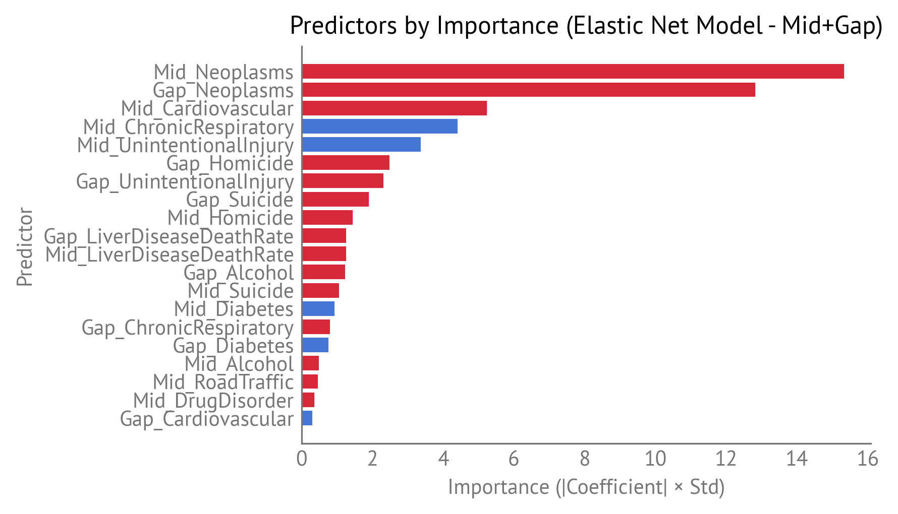
Predictors by importance.
The Neoplasms overall rate is the most important predictor, with an importance of 15.3. The Neoplasms gap is next, with an importance of 12.8.
When we aggregate importance by indicator (combining Mid and Gap predictors), we can see which health indicators matter most overall:
| Indicator | Mid_Importance | Gap_Importance | Total_Importance |
|---|---|---|---|
| Neoplasms | 15.3 | 12.8 | 28.2 |
| UnintentionalInjury | 3.37 | 2.31 | 5.69 |
| Cardiovascular | 5.24 | 0.306 | 5.55 |
| ChronicRespiratory | 4.42 | 0.801 | 5.22 |
| Homicide | 1.44 | 2.48 | 3.92 |
| Suicide | 1.05 | 1.9 | 2.96 |
| LiverDiseaseDeathRate | 1.26 | 1.26 | 2.52 |
| Alcohol | 0.491 | 1.23 | 1.73 |
| Diabetes | 0.934 | 0.755 | 1.69 |
| RoadTraffic | 0.468 | 0 | 0.468 |
| DrugDisorder | 0.363 | 0 | 0.363 |
The following figure visualizes indicator-level importance:
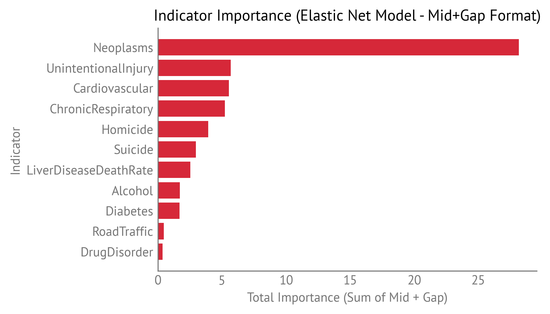
Indicator-level importance, showing which health indicators contribute most to explaining the HALE gender gap.
The top indicators are:
Neoplasms (total importance: 28.2) — Cancer is the dominant factor for HALE, with contributions from both the overall rate and the gender gap. Some part of the neoplasms gap is due to past smoking patterns, as men historically smoked more than women. Neoplasms gained importance after removing the childhood mortality indicator, suggesting it better captures its relationship with the HALE gap without that indicator.
Unintentional Injury (total importance: 5.69) — Unintentional injuries are the second most important factor, with contributions from both the overall rate and the gender gap. These injuries often show gender differences due to occupational exposures, risk-taking behaviors, and activity patterns.
Cardiovascular disease (total importance: 5.55) — Cardiovascular disease is the third most important factor, with contributions from both the overall rate and the gender gap. In many countries, cardiovascular disease rates are higher for women because cardiovascular risk increases with age, and women are more likely to live long enough to develop cardiovascular disease. Cardiovascular importance decreased after removing childhood mortality, suggesting some interaction between these indicators.
Chronic Respiratory disease (total importance: 5.22) — Chronic respiratory disease contributes substantially, with contributions from both the overall rate and the gender gap. Like neoplasms, some part of the Chronic Respiratory disease gap is due to past smoking patterns.
Homicide (total importance: 3.92) — Homicide contributes moderately, with contributions from both the overall rate and the gender gap. Homicide rates are typically much higher in men than women across most countries. Homicide gained substantial importance after removing the childhood mortality indicator, suggesting it may have been capturing some shared variance.
Suicide (total importance: 2.96) — Suicide contributes moderately, with contributions from both the overall rate and the gender gap. Suicide rates are typically much higher in men than women across most countries.
Liver Disease (total importance: 2.52) — Liver disease death rates contribute moderately, with contributions from both the overall rate and the gender gap. Liver disease is often related to alcohol consumption, but also includes non-alcoholic causes.
Alcohol (total importance: 1.73) — Alcohol use disorder death rates contribute moderately, with importance coming mostly from the gap component. The importance is lower than in previous analyses because the current model uses IHME data, which defines alcohol-related mortality more narrowly than WHO’s broader “alcohol-attributable” definition.
Diabetes (total importance: 1.69) — Diabetes contributes moderately, with contributions from both the overall rate and the gender gap. Diabetes gained importance after removing the childhood mortality indicator.
Residual
The following table shows country-level predictions and residuals:
| Country | Actual_HALE_Gap | Predicted_HALE_Gap | Residual | Abs_Residual |
|---|---|---|---|---|
| Germany | 0.862 | 1.67 | -0.803 | 0.803 |
| Sweden | 0.134 | 0.706 | -0.571 | 0.571 |
| Czechia | 3.09 | 2.55 | 0.537 | 0.537 |
| Austria | 1.36 | 1.84 | -0.472 | 0.472 |
| Chile | 1.41 | 1.81 | -0.399 | 0.399 |
| Slovakia | 3.93 | 3.57 | 0.359 | 0.359 |
| Belgium | 0.941 | 1.29 | -0.353 | 0.353 |
| Colombia | 2.89 | 2.56 | 0.329 | 0.329 |
| Canada | 1.25 | 0.938 | 0.317 | 0.317 |
| South Korea | 3.56 | 3.27 | 0.295 | 0.295 |
| Switzerland | 0.338 | 0.63 | -0.292 | 0.292 |
| Hungary | 3.72 | 3.43 | 0.292 | 0.292 |
| Japan | 2.93 | 2.64 | 0.29 | 0.29 |
| Portugal | 2.39 | 2.68 | -0.29 | 0.29 |
| Norway | 0.239 | -0.0397 | 0.278 | 0.278 |
| Latvia | 5.69 | 5.43 | 0.267 | 0.267 |
| Greece | 1.33 | 1.58 | -0.257 | 0.257 |
| Denmark | 0.895 | 0.651 | 0.244 | 0.244 |
| France | 1.82 | 1.6 | 0.222 | 0.222 |
| Lithuania | 6.06 | 6.27 | -0.206 | 0.206 |
| Australia | 1.16 | 0.994 | 0.166 | 0.166 |
| Mexico | 3.1 | 3.26 | -0.162 | 0.162 |
| Poland | 4.93 | 4.79 | 0.136 | 0.136 |
| New Zealand | 0.487 | 0.607 | -0.121 | 0.121 |
| United Kingdom | 0.695 | 0.582 | 0.112 | 0.112 |
| Italy | 1.07 | 0.964 | 0.108 | 0.108 |
| Luxembourg | 0.915 | 0.812 | 0.102 | 0.102 |
| Netherlands | 0.0186 | -0.0815 | 0.1 | 0.1 |
| Iceland | 0.16 | 0.26 | -0.0997 | 0.0997 |
| Türkiye | 1.17 | 1.26 | -0.0887 | 0.0887 |
| Spain | 1.52 | 1.61 | -0.084 | 0.084 |
| Israel | 0.611 | 0.548 | 0.0622 | 0.0622 |
| Costa Rica | 2.26 | 2.32 | -0.0588 | 0.0588 |
| Slovenia | 2.91 | 2.86 | 0.0519 | 0.0519 |
| Estonia | 4.79 | 4.83 | -0.0433 | 0.0433 |
| Ireland | 0.454 | 0.419 | 0.035 | 0.035 |
| Finland | 2.24 | 2.27 | -0.0275 | 0.0275 |
| United States | 1.8 | 1.78 | 0.0256 | 0.0256 |
The following figure shows residuals plotted against predicted values:
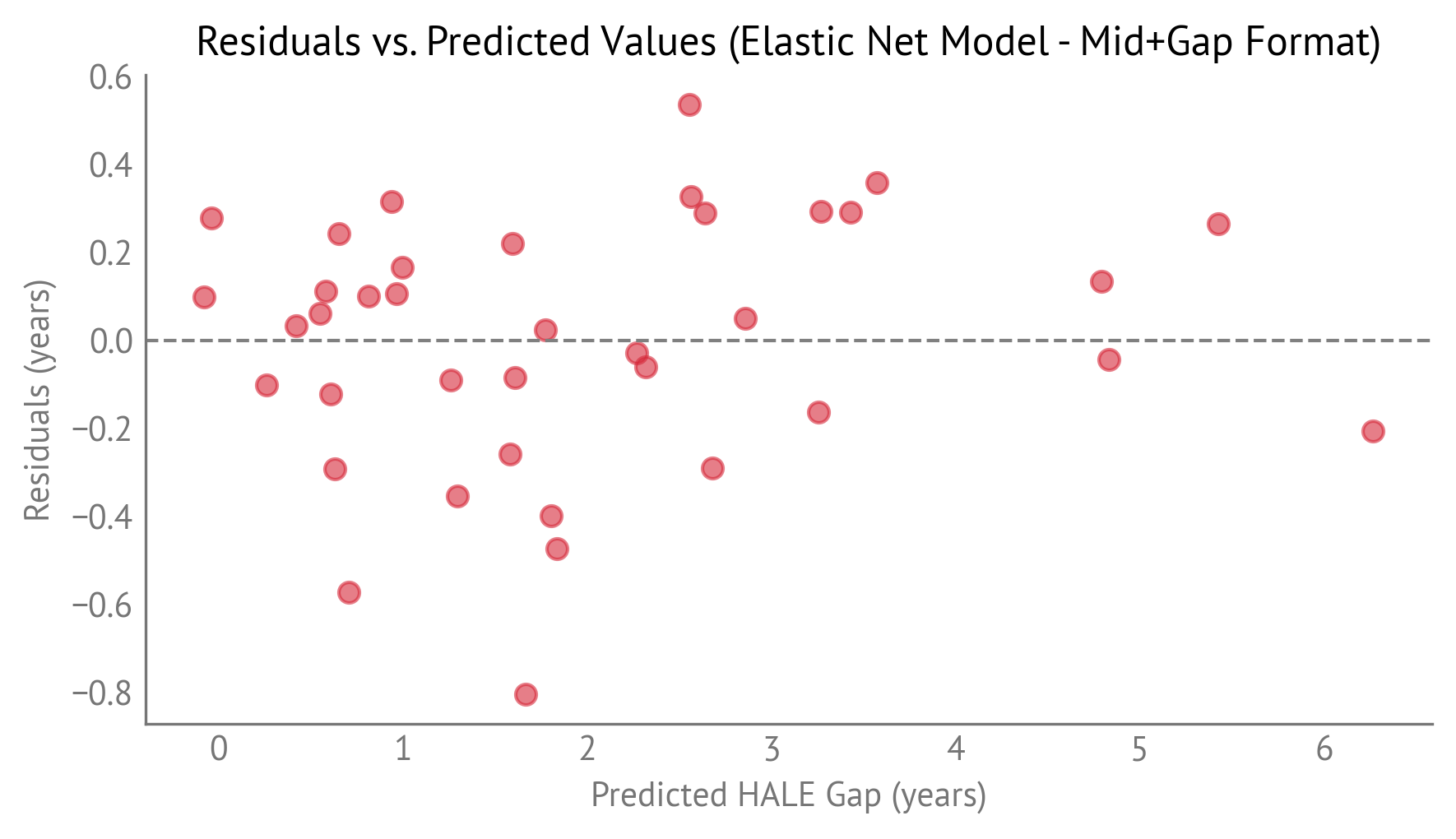
Residuals plotted against predicted HALE gap values.
The model shows good fit with no obvious systematic patterns in the residuals.
Comparison with Ordinary Least Squares
For comparison, we also fit an ordinary least squares (OLS) model using only the 20 predictors selected by Elastic Net. The following table compares performance:
| Model | R² | Adjusted R² | MAE | Number of Predictors | Non-Zero Coefficients |
|---|---|---|---|---|---|
| Elastic Net | 0.968 | 0.228 | 22 | 20 | |
| OLS (Selected Predictors) | 0.974 | 0.943 | 0.196 | 20 | 20 |
Both models perform similarly, with OLS achieving a slightly higher R² and lower MAE on the training data. However, the cross-validation R² of 0.78 for Elastic Net is a better estimate of out-of-sample performance and predictive validity.
Counterfactual Analysis
The methodology here is the same as for Life Expectancy.
The following table shows counterfactual results for the United States.
| Indicator | Current gap | Target gap | Target Country | Change in HALE gap |
|---|---|---|---|---|
| Neoplasms | 25.7 | 0 | -0.28 | |
| UnintentionalInjury | 5.26 | 0 | -0.0421 | |
| Cardiovascular | 19.4 | 0 | 0.00179 | |
| ChronicRespiratory | -5.82 | 0 | 0.0869 | |
| Homicide | 7.29 | 0 | -0.281 | |
| Suicide | 17.3 | 4.51 | Türkiye | -0.801 |
| LiverDiseaseDeathRate | 9.05 | 1.29 | Iceland | -0.205 |
| Alcohol | 5.54 | 0.306 | Colombia | -0.273 |
| Diabetes | 5.5 | 0 | 0.409 | |
| RoadTraffic | 11.2 | 2.04 | Iceland | -0.165 |
| DrugDisorder | 16 | 0.0226 | Japan | -0.206 |
The table is sorted by importance, which indicates in general how effective it is to reduce a particular gap. The counterfactual results (the “Change in HALE gap” column) indicate how much reducing that gap would specifically affect the HALE gap in the United States, which depends on how far the United States is from the target gap for that indicator.
The results show that reducing the Suicide gap from 17.3 to 4.51 (the level observed in Türkiye) would reduce the predicted HALE gap by 0.801 years, the largest single impact. Reducing the Neoplasms gap to zero would reduce the HALE gap by an additional 0.28 years. Reducing the Alcohol gap from 5.54 to 0.306 (the level observed in Colombia) would reduce the gap by 0.273 years. Reducing the Homicide gap to zero would reduce the gap by 0.281 years.
Most indicators show negative changes (gap-closing effects), but a few show positive changes (gap-widening effects). The positive changes occur when reducing a gap predictor would increase the HALE gap, which can happen when the relationship between predictors and the outcome is complex due to correlations among indicators.
When we sum the effects across all indicators, we can see the total potential impact:
Gap-closing indicators (negative changes): The sum of all indicators that would reduce the HALE gap includes Suicide (-0.801), Neoplasms (-0.28), Alcohol (-0.273), Homicide (-0.281), Liver Disease (-0.205), Drug Disorder (-0.206), Road Traffic (-0.165), and Unintentional Injury (-0.042), for a total reduction of -2.25 years.
Gap-widening indicators (positive changes): The sum of all indicators that would increase the HALE gap includes Diabetes (+0.409) and Chronic Respiratory disease (+0.087), for a total increase of +0.50 years.
The net effect of closing all gaps to their target levels would be a reduction in the predicted HALE gap. This represents a substantial part of the current gap.
Comparison of Life Expectancy and HALE Results
The Life Expectancy model performs better than the HALE model:
Life Expectancy: Cross-validation R² of 0.879, MAE of 0.326 years
HALE: Cross-validation R² of 0.778, MAE of 0.422 years
The lower performance for HALE may reflect the additional complexity of modeling healthy years, which depends on both mortality and morbidity patterns, whereas Life Expectancy depends entirely on mortality.
Both models select a similar number of predictors:
Life Expectancy: 13 out of 22 predictors (59%)
HALE: 20 out of 22 predictors (91%)
The HALE model uses more predictors, suggesting that more factors are relevant for explaining healthy life expectancy than overall life expectancy.
The relative importance of indicators differs between the two models:
Life Expectancy:
Neoplasms (11.4) — entirely from the gap component
Unintentional Injury (4.93) — entirely from the gap component
Chronic Respiratory disease (2.22) — from both overall rate and gap
Liver Disease (2.08) — mostly from the gap component
Homicide (1.84) — from both overall rate and gap
Suicide (1.82) — entirely from the gap component
Alcohol (1.53) — mostly from the gap component
HALE:
Neoplasms (28.2) — from both overall rate and gap
Cardiovascular disease (5.55) — from both overall rate and gap
Unintentional Injury (5.69) — from both overall rate and gap
Chronic Respiratory disease (5.22) — from both overall rate and gap
Homicide (3.92) — from both overall rate and gap
Suicide (2.96) — from both overall rate and gap
Liver Disease (2.52) — from both overall rate and gap
Alcohol (1.73) — mostly from the gap component
Diabetes (1.69) — from both overall rate and gap
Neoplasms (cancer) is the most important factor in both models, but its relative importance is much higher for HALE. Cardiovascular disease is important for HALE but was not selected for Life Expectancy. Alcohol has lower importance in both models than in previous analyses, reflecting the use of IHME data which defines alcohol-related mortality more narrowly.
The counterfactual analysis shows that Suicide has the largest single impact in both models, followed by Neoplasms and Alcohol. The patterns are similar but the magnitudes differ between the two outcomes.
Implications
These differences suggest that:
Cancer prevention and treatment is the most important factor for both outcomes, but particularly critical for healthy life expectancy, as neoplasms have much higher importance for HALE (28.2) than for Life Expectancy (11.4).
Cardiovascular disease affects healthy years (importance 5.55 for HALE) but was not selected as a predictive factor for total life expectancy, suggesting it may have different relationships with mortality versus healthy years.
Suicide prevention has substantial importance in both models and shows the largest counterfactual impact, suggesting it is a critical intervention target.
Unintentional injuries are important for both outcomes, ranking second for Life Expectancy and third for HALE.
Alcohol-related interventions remain important but have lower importance than in previous analyses, reflecting the use of IHME data which defines alcohol-related mortality more narrowly than WHO’s broader “alcohol-attributable” definition.