The empiricaldist API

The empiricaldist API#

This notebook documents the most useful features of the empiricaldist API.

Click here to run this notebook on Colab.

try:
    import empiricaldist
except ImportError:
    !pip install empiricaldist

import numpy as np
import pandas as pd
import matplotlib.pyplot as plt

A Pmf is a Series#

empiricaldist provides Pmf, which is a Pandas Series that represents a probability mass function.

from empiricaldist import Pmf

You can create a Pmf in any of the ways you can create a Series, but the most common way is to use from_seq to make a Pmf from a sequence.

The following is a Pmf that represents a six-sided die.

d6 = Pmf.from_seq([1,2,3,4,5,6])

By default, the probabilities are normalized to add up to 1.

d6

	probs
1	0.166667
2	0.166667
3	0.166667
4	0.166667
5	0.166667
6	0.166667

But you can also make an unnormalized Pmf if you want to keep track of the counts.

d6 = Pmf.from_seq([1,2,3,4,5,6], normalize=False)
d6

	probs
1	1
2	1
3	1
4	1
5	1
6	1

Or normalize later (the return value is the prior sum).

d6.normalize()

Now the Pmf is normalized.

d6

	probs
1	0.166667
2	0.166667
3	0.166667
4	0.166667
5	0.166667
6	0.166667

Properties#

In a Pmf the index contains the quantities (qs) and the values contain the probabilities (ps).

These attributes are available as properties that return arrays (same semantics as the Pandas values property)

d6.qs

array([1, 2, 3, 4, 5, 6])

d6.ps

array([0.16666667, 0.16666667, 0.16666667, 0.16666667, 0.16666667,
       0.16666667])

Plotting PMFs#

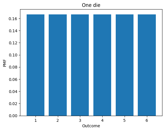
Pmf provides two plotting functions. bar plots the Pmf as a histogram.

def decorate_dice(title):
    """Labels the axes.
    
    title: string
    """
    plt.xlabel('Outcome')
    plt.ylabel('PMF')
    plt.title(title)

d6.bar()
decorate_dice('One die')

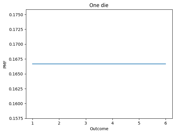
_images/f79acfe2788a50bf93cc7ccfd04ab7c91a7439b34e8a2e77939f93f18a2f52f8.png

plot displays the Pmf as a line.

d6.plot()
decorate_dice('One die')

_images/861fe5d417414f70d2c8cb6fb2cc6838a4bff8f0eb0c0e787717852edccbc519.png

Selection#

The bracket operator looks up an outcome and returns its probability.

d6[1]

0.16666666666666666

d6[6]

0.16666666666666666

Outcomes that are not in the distribution cause a KeyError

d6[7]

You can also use parentheses to look up a quantity and get the corresponding probability.

d6(1)

0.16666666666666666

With parentheses, a quantity that is not in the distribution returns 0, not an error.

d6(7)

Mutation#

Pmf objects are mutable, but in general the result is not normalized.

d7 = d6.copy()

d7[7] = 1/6
d7

	probs
1	0.166667
2	0.166667
3	0.166667
4	0.166667
5	0.166667
6	0.166667
7	0.166667

d7.sum()

1.1666666666666665

d7.normalize()

1.1666666666666665

d7.sum()

1.0000000000000002

Statistics#

Pmf overrides the statistics methods to compute mean, median, etc.

These functions only work correctly if the Pmf is normalized.

d6 = Pmf.from_seq([1,2,3,4,5,6])

d6.mean()

3.5

d6.var()

2.9166666666666665

d6.std()

1.707825127659933

Sampling#

choice chooses a random values from the Pmf, following the API of np.random.choice

d6.choice(size=10)

array([3, 4, 2, 4, 2, 3, 5, 4, 1, 5])

sample chooses a random values from the Pmf, with replacement.

d6.sample(n=10)

array([5., 3., 4., 3., 5., 3., 1., 2., 4., 3.])

CDFs#

empiricaldist also provides Cdf, which represents a cumulative distribution function.

from empiricaldist import Cdf

You can create an empty Cdf and then add elements.

Here’s a Cdf that represents a four-sided die.

d4 = Cdf.from_seq([1,2,3,4])

d4

	probs
1	0.25
2	0.50
3	0.75
4	1.00

Properties#

In a Cdf the index contains the quantities (qs) and the values contain the probabilities (ps).

These attributes are available as properties that return arrays (same semantics as the Pandas values property)

d4.qs

array([1, 2, 3, 4])

d4.ps

array([0.25, 0.5 , 0.75, 1.  ])

Displaying CDFs#

Cdf provides two plotting functions.

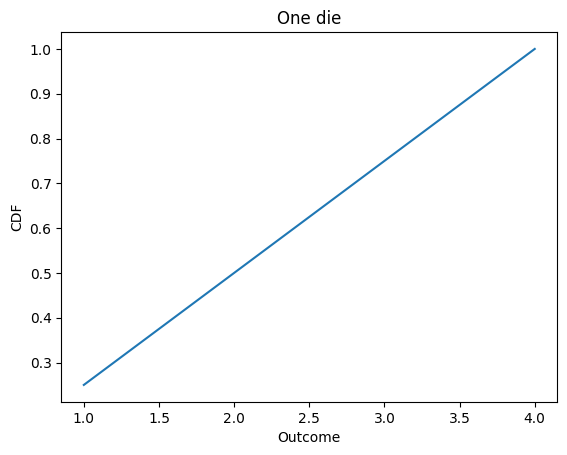
plot displays the Cdf as a line.

def decorate_dice(title):
    """Labels the axes.
    
    title: string
    """
    plt.xlabel('Outcome')
    plt.ylabel('CDF')
    plt.title(title)

d4.plot()
decorate_dice('One die')

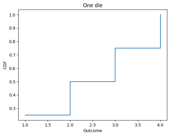
_images/902042f123cbcff5a599a52e4ad12cce681771ae6912f57edee3979b8aa4a3a1.png

step plots the Cdf as a step function (which is more technically correct).

d4.step()
decorate_dice('One die')

_images/5a20d538f758dfaea11d40426b8c9855171a8bc9c61e9573c04348bc5f300e42.png

Selection#

The bracket operator works as usual.

d4[1]

0.25

d4[4]

1.0

Evaluating CDFs#

Cdf provides forward and inverse, which evaluate the CDF and its inverse as functions.

Evaluating a Cdf forward maps from a quantity to its cumulative probability.

d6 = Cdf.from_seq([1,2,3,4,5,6])

d6.forward(3)

array(0.5)

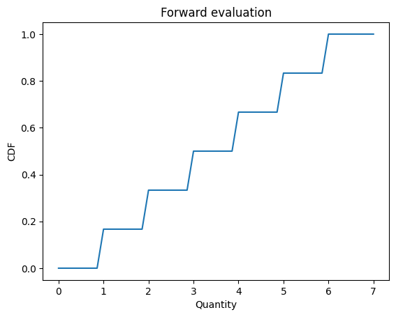
forward interpolates, so it works for quantities that are not in the distribution.

d6.forward(3.5)

array(0.5)

d6.forward(0)

array(0.)

d6.forward(7)

array(1.)

You can also call the Cdf like a function (which it is).

d6(1.5)

array(0.16666667)

forward can take an array of quantities, too.

def decorate_cdf(title):
    """Labels the axes.
    
    title: string
    """
    plt.xlabel('Quantity')
    plt.ylabel('CDF')
    plt.title(title)

qs = np.linspace(0, 7)
ps = d6(qs)
plt.plot(qs, ps)
decorate_cdf('Forward evaluation')

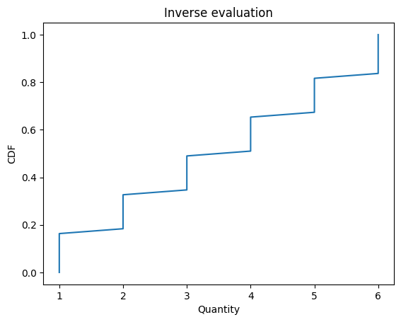
_images/6e53db21789ec80f502bfe3ebd029f21c23d16b1c4107b84444aa261f76567e6.png

Cdf also provides inverse, which computes the inverse Cdf:

d6.inverse(0.5)

array(3.)

quantile is a synonym for inverse

d6.quantile(0.5)

array(3.)

inverse and quantile work with arrays

ps = np.linspace(0, 1)
qs = d6.quantile(ps)
plt.plot(qs, ps)
decorate_cdf('Inverse evaluation')

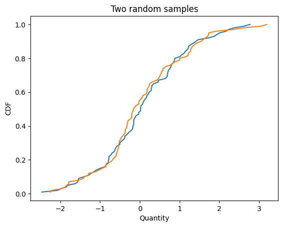
_images/126ff61c8d1b9e98b52ba75b379fbef43201f89ac9129ea7c3244f305c19c1fa.png

These functions provide a simple way to make a Q-Q plot.

Here are two samples from the same distribution.

cdf1 = Cdf.from_seq(np.random.normal(size=100))
cdf2 = Cdf.from_seq(np.random.normal(size=100))

cdf1.plot()
cdf2.plot()
decorate_cdf('Two random samples')

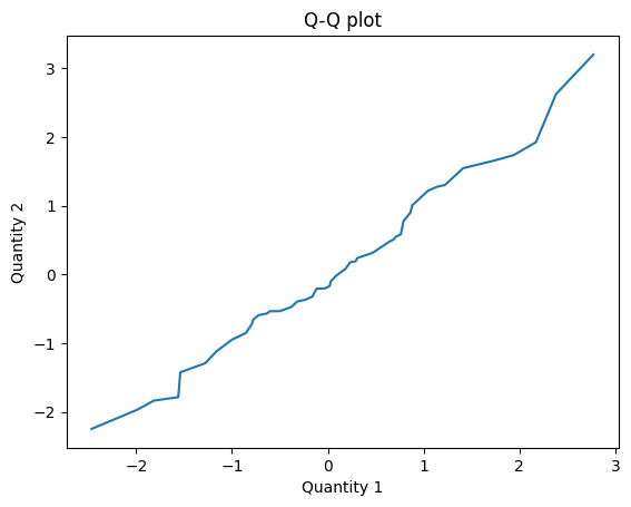
_images/31d4a30c64a4662a20cbea62d2531efb81582f9b84d89ab42b9874bfa1d07277.png

Here’s how we compute the Q-Q plot.

def qq_plot(cdf1, cdf2):
    """Compute results for a Q-Q plot.
    
    Evaluates the inverse Cdfs for a 
    range of cumulative probabilities.
    
    cdf1: Cdf
    cdf2: Cdf
    
    Returns: tuple of arrays
    """
    ps = np.linspace(0, 1)
    q1 = cdf1.quantile(ps)
    q2 = cdf2.quantile(ps)
    return q1, q2

The result is near the identity line, which suggests that the samples are from the same distribution.

q1, q2 = qq_plot(cdf1, cdf2)
plt.plot(q1, q2)
plt.xlabel('Quantity 1')
plt.ylabel('Quantity 2')
plt.title('Q-Q plot');

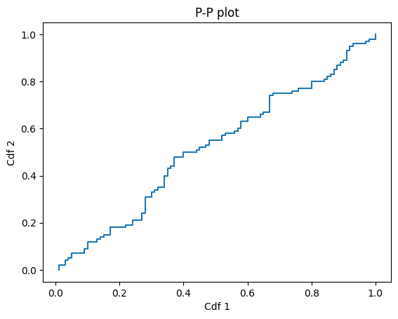
_images/a4064fe737da998350ed39117f5b9afe24036e2a41524a07d7b5af98105bb33a.png

Here’s how we compute a P-P plot

def pp_plot(cdf1, cdf2):
    """Compute results for a P-P plot.
    
    Evaluates the Cdfs for all quantities in either Cdf.
    
    cdf1: Cdf
    cdf2: Cdf
    
    Returns: tuple of arrays
    """
    qs = cdf1.index.union(cdf2.index)
    p1 = cdf1(qs)
    p2 = cdf2(qs)
    return p1, p2

And here’s what it looks like.

p1, p2 = pp_plot(cdf1, cdf2)
plt.plot(p1, p2)
plt.xlabel('Cdf 1')
plt.ylabel('Cdf 2')
plt.title('P-P plot');

_images/f6356576caaaf07bddf4513f55ed6dc4bef8c8d3287a1cde8e6fed81609f8a78.png

Mutation#

Cdf objects are mutable, but in general the result is not a valid Cdf.

d4[5] = 1.25
d4

	probs
1	0.25
2	0.50
3	0.75
4	1.00
5	1.25

d4.normalize()
d4

	probs
1	0.2
2	0.4
3	0.6
4	0.8
5	1.0

Statistics#

Cdf overrides the statistics methods to compute mean, median, etc.

d6.mean()

3.5

d6.var()

2.916666666666667

d6.std()

1.7078251276599332

Sampling#

choice chooses a random values from the Cdf, following the API of np.random.choice

d6.choice(size=10)

array([1, 1, 3, 2, 3, 4, 4, 5, 2, 2])

sample chooses a random values from the Cdf, with replacement.

d6.sample(n=10)

array([4., 3., 2., 6., 5., 4., 1., 6., 1., 4.])

Arithmetic#

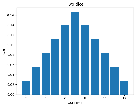
Pmf and Cdf provide add_dist, which computes the distribution of the sum.

Here’s the distribution of the sum of two dice.

d6 = Pmf.from_seq([1,2,3,4,5,6])

twice = d6.add_dist(d6)
twice

	probs
2	0.027778
3	0.055556
4	0.083333
5	0.111111
6	0.138889
7	0.166667
8	0.138889
9	0.111111
10	0.083333
11	0.055556
12	0.027778

twice.bar()
decorate_dice('Two dice')
twice.mean()

6.999999999999998

_images/431e6faa4a04d1077a1eef79877f75d9ff93ec24c92c00f240f55dde8e898944.png

To add a constant to a distribution, you could construct a deterministic Pmf

const = Pmf.from_seq([1])
d6.add_dist(const)

	probs
2	0.166667
3	0.166667
4	0.166667
5	0.166667
6	0.166667
7	0.166667

But add_dist also handles constants as a special case:

d6.add_dist(1)

	probs
2	0.166667
3	0.166667
4	0.166667
5	0.166667
6	0.166667
7	0.166667

Other arithmetic operations are also implemented

d4 = Pmf.from_seq([1,2,3,4])

d6.sub_dist(d4)

	probs
-3	0.041667
-2	0.083333
-1	0.125000
0	0.166667
1	0.166667
2	0.166667
3	0.125000
4	0.083333
5	0.041667

d4.mul_dist(d4)

	probs
1	0.0625
2	0.1250
3	0.1250
4	0.1875
6	0.1250
8	0.1250
9	0.0625
12	0.1250
16	0.0625

d4.div_dist(d4)

	probs
0.250000	0.0625
0.333333	0.0625
0.500000	0.1250
0.666667	0.0625
0.750000	0.0625
1.000000	0.2500
1.333333	0.0625
1.500000	0.0625
2.000000	0.1250
3.000000	0.0625
4.000000	0.0625

Comparison operators#

Pmf implements comparison operators that return probabilities.

You can compare a Pmf to a scalar:

d6.lt_dist(3)

0.3333333333333333

d4.ge_dist(2)

0.75

Or compare Pmf objects:

d4.gt_dist(d6)

0.25

d6.le_dist(d4)

0.41666666666666663

d4.eq_dist(d6)

0.16666666666666666

Interestingly, this way of comparing distributions is nontransitive.

A = Pmf.from_seq([2, 2, 4, 4, 9, 9])
B = Pmf.from_seq([1, 1, 6, 6, 8, 8])
C = Pmf.from_seq([3, 3, 5, 5, 7, 7])

A.gt_dist(B)

0.5555555555555556

B.gt_dist(C)

0.5555555555555556

C.gt_dist(A)

0.5555555555555556

Joint distributions#

Pmf.make_joint takes two Pmf objects and makes their joint distribution, assuming independence.

d4 = Pmf.from_seq(range(1,5))
d4

	probs
1	0.25
2	0.25
3	0.25
4	0.25

d6 = Pmf.from_seq(range(1,7))
d6

	probs
1	0.166667
2	0.166667
3	0.166667
4	0.166667
5	0.166667
6	0.166667

joint = Pmf.make_joint(d4, d6)
joint

		probs
1	1	0.041667
	2	0.041667
	3	0.041667
	4	0.041667
	5	0.041667
	6	0.041667
2	1	0.041667
	2	0.041667
	3	0.041667
	4	0.041667
	5	0.041667
	6	0.041667
3	1	0.041667
	2	0.041667
	3	0.041667
	4	0.041667
	5	0.041667
	6	0.041667
4	1	0.041667
	2	0.041667
	3	0.041667
	4	0.041667
	5	0.041667
	6	0.041667

The result is a Pmf object that uses a MultiIndex to represent the values.

joint.index

MultiIndex([(1, 1),
            (1, 2),
            (1, 3),
            (1, 4),
            (1, 5),
            (1, 6),
            (2, 1),
            (2, 2),
            (2, 3),
            (2, 4),
            (2, 5),
            (2, 6),
            (3, 1),
            (3, 2),
            (3, 3),
            (3, 4),
            (3, 5),
            (3, 6),
            (4, 1),
            (4, 2),
            (4, 3),
            (4, 4),
            (4, 5),
            (4, 6)],
           )

If you ask for the qs, you get an array of pairs:

joint.qs

array([(1, 1), (1, 2), (1, 3), (1, 4), (1, 5), (1, 6), (2, 1), (2, 2),
       (2, 3), (2, 4), (2, 5), (2, 6), (3, 1), (3, 2), (3, 3), (3, 4),
       (3, 5), (3, 6), (4, 1), (4, 2), (4, 3), (4, 4), (4, 5), (4, 6)],
      dtype=object)

You can select elements using tuples:

joint[1,1]

0.041666666666666664

You can get unnnormalized conditional distributions by selecting on different axes:

Pmf(joint[1])

	probs
1	0.041667
2	0.041667
3	0.041667
4	0.041667
5	0.041667
6	0.041667

Pmf(joint.loc[:, 1])

	probs
1	0.041667
2	0.041667
3	0.041667
4	0.041667

But Pmf also provides conditional(i, val) which returns the conditional distribution where variable i has the value val:

joint.conditional(0, 1)

	probs
1	0.166667
2	0.166667
3	0.166667
4	0.166667
5	0.166667
6	0.166667

joint.conditional(1, 1)

	probs
1	0.25
2	0.25
3	0.25
4	0.25

It also provides marginal(i), which returns the marginal distribution along axis i

joint.marginal(0)

	probs
1	0.25
2	0.25
3	0.25
4	0.25

joint.marginal(1)

	probs
1	0.166667
2	0.166667
3	0.166667
4	0.166667
5	0.166667
6	0.166667

Here are some ways of iterating through a joint distribution.

for q in joint.qs:
    print(q)

(1, 1)
(1, 2)
(1, 3)
(1, 4)
(1, 5)
(1, 6)
(2, 1)
(2, 2)
(2, 3)
(2, 4)
(2, 5)
(2, 6)
(3, 1)
(3, 2)
(3, 3)
(3, 4)
(3, 5)
(3, 6)
(4, 1)
(4, 2)
(4, 3)
(4, 4)
(4, 5)
(4, 6)

for p in joint.ps:
    print(p)

041666666666666664
041666666666666664
041666666666666664
041666666666666664
041666666666666664
041666666666666664
041666666666666664
041666666666666664
041666666666666664
041666666666666664
041666666666666664
041666666666666664
041666666666666664
041666666666666664
041666666666666664
041666666666666664
041666666666666664
041666666666666664
041666666666666664
041666666666666664
041666666666666664
041666666666666664
041666666666666664
041666666666666664

for q, p in joint.items():
    print(q, p)

(1, 1) 0.041666666666666664
(1, 2) 0.041666666666666664
(1, 3) 0.041666666666666664
(1, 4) 0.041666666666666664
(1, 5) 0.041666666666666664
(1, 6) 0.041666666666666664
(2, 1) 0.041666666666666664
(2, 2) 0.041666666666666664
(2, 3) 0.041666666666666664
(2, 4) 0.041666666666666664
(2, 5) 0.041666666666666664
(2, 6) 0.041666666666666664
(3, 1) 0.041666666666666664
(3, 2) 0.041666666666666664
(3, 3) 0.041666666666666664
(3, 4) 0.041666666666666664
(3, 5) 0.041666666666666664
(3, 6) 0.041666666666666664
(4, 1) 0.041666666666666664
(4, 2) 0.041666666666666664
(4, 3) 0.041666666666666664
(4, 4) 0.041666666666666664
(4, 5) 0.041666666666666664
(4, 6) 0.041666666666666664

for (q1, q2), p in joint.items():
    print(q1, q2, p)

1 0.041666666666666664
2 0.041666666666666664
3 0.041666666666666664
4 0.041666666666666664
5 0.041666666666666664
6 0.041666666666666664
1 0.041666666666666664
2 0.041666666666666664
3 0.041666666666666664
4 0.041666666666666664
5 0.041666666666666664
6 0.041666666666666664
1 0.041666666666666664
2 0.041666666666666664
3 0.041666666666666664
4 0.041666666666666664
5 0.041666666666666664
6 0.041666666666666664
1 0.041666666666666664
2 0.041666666666666664
3 0.041666666666666664
4 0.041666666666666664
5 0.041666666666666664
6 0.041666666666666664

BSD 3-clause license: https://opensource.org/licenses/BSD-3-Clause

The empiricaldist API

Contents

The empiricaldist API#

A Pmf is a Series#

Properties#

Plotting PMFs#

Selection#

Mutation#

Statistics#

Sampling#

CDFs#

Properties#

Displaying CDFs#

Selection#

Evaluating CDFs#

Mutation#

Statistics#

Sampling#

Arithmetic#

Comparison operators#

Joint distributions#