Think Linear Algebra is not for sale yet, but if you would like to support this project, you can buy me a coffee.
3. Projection#
This chapter is about one of the most important ideas in linear algebra, projection, and the operation that computes it, the dot product.
To sneak up on the idea of projection, we’ll start by converting a vector from Cartesian to polar coordinates and back. From there, we’ll define projection geometrically and compute it with polar coordinates. Then we’ll compute it again in Cartesian coordinates, and show the the result is the dot product.
We’ll take a small detour to construct a rotation matrix and use it to compute perpendicular vectors. And then, to apply what we’ve learned, we’ll play pool!
Click here to run this notebook on Colab.
Show code cell content
%load_ext autoreload
%autoreload 2
Show code cell content
from os.path import basename, exists


def download(url):
    filename = basename(url)
    if not exists(filename):
        from urllib.request import urlretrieve

        local, _ = urlretrieve(url, filename)
        print("Downloaded " + local)


download("https://github.com/AllenDowney/ThinkLinearAlgebra/raw/main/utils.py")
Show code cell content
import numpy as np
import pandas as pd
import matplotlib.pyplot as plt

from utils import decorate, remove_spines
from utils import plot_vector, plot_vectors, plot_rejection
from utils import set_precision

set_precision(4)
3.1. Polar Coordinates#
Let’s start with a two-dimensional vector with Cartesian coordinates x and y.
x, y = 1.2, 2.7
a = np.array([x, y])
a
array([1.2, 2.7])
Here’s the graphical representation of this vector as an arrow with its tail at the origin and its head at the point \((x, y)\).
from utils import plot_angle_between, decorate_plane

plot_vector(a)
plt.plot([0, x, x], [0, 0, y], ':', color='gray')
plot_angle_between([1, 0], a, radius=0.25)
lim = [-0.1, 3.1]
decorate_plane(lim=lim)
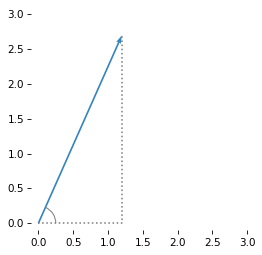
To compute the length of this vector, we can use the Pythagorean formula to compute the hypotenuse of a right triangle with side lengths \(x\) and \(y\).
x, y = a
np.sqrt(x**2 + y**2)
2.9547
Or the hypot function does the same thing.
np.hypot(x, y)
2.9547
The length of a vector is called its norm. More precisely, the length we computed is the 2-norm, because we squared the components before adding them up. NumPy provides a function that computes norms.
from numpy.linalg import norm

norm(a)
2.9547
To represent the direction of the vector, we’ll use the angle it forms with the positive \(x\) axis, which we can compute using the inverse tangent function, arctan2.
phi = np.arctan2(y, x)
phi
1.1526
The length and angle we just computed represent the vector in polar coordinates. We’ll use the following function to convert from Cartesian to polar coordinates.
def cart2pol(v):
    x, y = np.transpose(v)
    r = np.hypot(x, y)
    phi = np.arctan2(y, x)
    return r, phi
Here’s the polar representation of a.
r, phi = cart2pol(a)
r, phi
(2.9547, 1.1526)
The polar representation makes it easier to perform certain computations – one example is projection.
3.2. Projection With Polar Coordinates#
We’ll start by computing the scalar projection of a onto the \(x\) axis, which you can think of as the shadow a would cast on the \(x\) axis if lighted from above.
By the rules of trigonometry, we can compute it like this.
scalar_proj_x = r * np.cos(phi)
scalar_proj_x
1.2000
Similarly, we can compute the projection of a onto the \(y\) axis.
scalar_proj_y = r * np.sin(phi)
scalar_proj_y
2.7000
These scalar projections are the coordinates of a.
So we have found a way to convert polar to Cartesian coordinates, which we can wrap in a function.
def pol2cart(r, phi):
    return r * np.array([np.cos(phi), np.sin(phi)])
And confirm that we get back the vector we started with.
pol2cart(r, phi)
array([1.2, 2.7])
So far, we converted a from Cartesian to polar coordinates and then back to Cartesian coordinates.
Now let’s do something more useful, projecting one vector onto another.
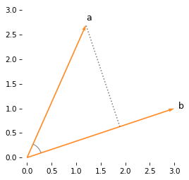
To demonstrate, here’s another vector, b, in Cartesian coordinates.
b = np.array([3, 1])
Here’s a graphical representation of a and b, and a dotted line that shows a perpendicular dropped from a onto b.
Where this perpendicular lands on b is the projection of a on b.
plot_vectors([a, b], color='C1', labels='ab')
plot_angle_between(b, a, radius=0.3)
plot_rejection(a, b)
decorate_plane(lim=lim)
One way to compute this projection is to find the angle between a and b, and use trigonometry to compute the length of the projection.
To find the angle, we’ll convert b and a to polar coordinates.
rs, phis = cart2pol([b, a])
phis
array([0.3218, 1.1526])
phis contains two angles: from b to the \(x\) axis, and from a to the \(x\) axis.
The difference is the angle between them.
np.diff(phis)
array([0.8308])
So we can use this function to compute the angle between two vectors.
def angle_between(a, b):
    rs, phis = cart2pol([a, b])
    return np.diff(phis)
theta = angle_between(b, a)
theta
array([0.8308])
If you look again at the previous figure, you’ll see that theta is the angle of a right triangle whose hypotenuse is the length of a.
So the length of the adjacent side is \(\|a\| \cos \theta\).
comp_a_on_b = norm(a) * np.cos(theta)
comp_a_on_b
array([1.9922])
This result is the scalar projection of a on b, also called the component of a in the direction of b.
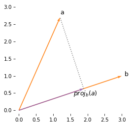
If we can multiply the scalar projection by a unit vector in the direction of b, the result is the vector projection of a on b.
b_hat = b / norm(b)
proj_a_on_b = comp_a_on_b * b_hat
proj_a_on_b
array([1.89, 0.63])
The following figure shows this vector projection.
plot_vectors([a, b], color='C1', labels='ab')
plot_rejection(a, b)
plot_vector(proj_a_on_b, color='C4', alpha=0.9, label='$proj_b(a)$', label_pos=1)
decorate_plane(lim=lim)
To summarize, if we have vectors in polar coordinates, we can compute the projection of one vector onto the other by computing the angle between them and using trigonometry.
But what if we have vectors in Cartesian coordinates?
3.3. Projection With Cartesian Coordinates#
If we have a and b in Cartesian coordinates, we can compute the projection of a on b by converting both to polar coordinates, subtracting their angles, and computing \(\|a\| \cos \phi\)
But there’s a better way, which we’ll discover with some help from SymPy.
Let’s define symbolic versions of the vectors b and a.
import sympy as sp

ax, ay, bx, by = sp.symbols('a_x a_y b_x b_y', real=True)

a_sym = sp.Matrix([ax, ay])
b_sym = sp.Matrix([bx, by])
b_sym
And convert them to polar coordinates.
r_a = a_sym.norm()
phi_a = sp.atan2(ay, ax)

r_b = b_sym.norm()
phi_b = sp.atan2(by, bx)
Here’s the length of b.
r_b
And its angle.
phi_b
Now we can compute the scalar projection of a onto b.
proj_expr = r_a * sp.cos(phi_b - phi_a)
proj_expr
This expression applies a trig function (cosine) to the inverse of another trig function (tangent) – which suggests that there might be a simpler form. Fortunately, SymPy knows the trigonometric identities, and it can simplify the expression.
proj_expr.simplify()
The numerator of this expression is the dot product of a and b, and the denominator is the norm of b.
So we can compute the scalar projection like this.
b_sym.dot(a_sym) / b_sym.norm()
In math notation, the scalar projection of \(a\) on \(b\) is
Let’s put that in a function we can use with NumPy arrays.
def scalar_projection(a, b):
    return np.dot(a, b) / norm(b)
If we test it with a and b, the result is what we got using polar coordinates.
comp_a_on_b = scalar_projection(a, b)
comp_a_on_b
1.9922
To get the vector projection, we’ll multiply the scalar projection by a unit vector in the direction of b.
The unit vector is called b_hat because in math notation we use a “hat” (actually a caret) to indicate a unit vector, like \(\hat{b}\).
def vector_projection(a, b):
    b_hat = b / norm(b)
    return scalar_projection(a, b) * b_hat
And the result is what we got using polar coordinates.
proj_a_on_b = vector_projection(a, b)
proj_a_on_b
array([1.89, 0.63])
The dot product is commutative, so b @ a and a @ b are the same.
np.allclose(b @ a, a @ b)
True
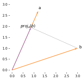
But scalar projection is not commutative, so the projection of b onto a is not the same as the projection of a onto b.
scalar_projection(b, a), scalar_projection(a, b)
(2.1322, 1.9922)
The following figure shows the projection of b onto a, which is not the same length or direction as the projection of a onto b.
proj_b_on_a = vector_projection(b, a)
plot_vectors([a, b], color='C1', labels='ab')
plot_rejection(b, a)
plot_vector(proj_b_on_a, color='C4', alpha=0.9, label='$proj_a(b)$', label_pos=11)
decorate_plane(lim=lim)
In summary, using polar coordinates and trigonometry, we found that we can write the scalar projection of \(a\) onto \(b\):
where \(\theta\) is the angle between the vectors. With some help from SymPy, we proved that we can also compute the scalar projection using Cartesian coordinates:
Setting the right sides equal, and multiplying through by the norm of \(b\), we have
If \(a\) and \(b\) point in the same direction, \(\theta=0\), so \(\cos \theta = 1\), and the dot product is the product of the lengths of the vectors.
If \(a\) and \(b\) are perpendicular, \(\cos \theta = 0\), and the dot product is 0.
3.4. Vector Rejection#
In some of the previous figures, I used a function called plot_rejection to draw a perpendicular line dropped from one vector to another.
That perpendicular is called the vector rejection because it represents the component of the vector that’s left over (rejected) if we subtract the vector projection.
In the example, we have computed the projection of a on b.
proj_a_on_b
array([1.89, 0.63])
So we can compute the rejection like this:
rej_a_on_b = a - proj_a_on_b
Here’s what it looks like:
plot_vectors([a, b], color='C1', labels='ab')
plot_vector(proj_a_on_b, color='C4', alpha=0.9, label='$proj_b(a)$', label_pos=1)
plot_vector(rej_a_on_b, proj_a_on_b, color='C4', alpha=0.9, label='$rej_b(a)$', label_pos=2)
decorate_plane(lim=lim)
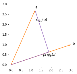
We can see that the original vector, a, is the sum of the projection and rejection.
The following function computes the vector rejection of a from b.
def vector_rejection(a, b):
    return a - vector_projection(a, b)
We will use vector projection and rejection again when we get to the pool example.
3.5. Rotation#
In previous sections we computed the projection of one vector on another by converting to polar coordinates. Then we used SymPy to work out the same operation with Cartesian coordinates. Now we’ll use the same method to rotate a vector – and use it to find a perpendicular vector.
Suppose we want to rotate a vector counter-clockwise by angle theta (in radians).
theta = sp.symbols('theta')
theta
Since we already have the vector b in symbolic form, we’ll use it again.
b_sym
We’ll convert it to polar coordinates.
r_b = b_sym.norm()
phi_b = sp.atan2(by, bx)
Now we can add theta to the angle of b and convert back to Cartesian coordinates.
x = r_b * sp.cos(phi_b + theta)
x
y = r_b * sp.sin(phi_b + theta)
y
Since those expressions contain sums of angles, we’ll use the expand_trig function to expand the trigonometric functions and then simplify to compact them.
sp.expand_trig(x).simplify()
sp.expand_trig(y).simplify()
We can see that the coordinates of the rotated vector can be computed as a weighted sum of \(b_x\) and \(b_y\). So if we put the weights in a matrix, we can express vector rotation using matrix multiplication. Here’s the rotation matrix.
R = sp.Matrix([[sp.cos(theta), -sp.sin(theta)],
               [sp.sin(theta),  sp.cos(theta)]])

R
And here’s the result when we multiply by \(b\).
R @ b_sym
We will use rotation matrices several times in later chapters.
3.6. Finding a Perpendicular#
We can use rotation to find a vector perpendicular to \(b\), by rotating counter-clockwise by 90 degrees – or \(\pi/2\) radians.
We’ll use this dictionary to substitute \(\pi/2\) for theta.
subs = {theta: sp.pi / 2}
subs
{theta: pi/2}
When we substitute into the rotation matrix, the result is pleasingly simple.
R_90 = R.subs(subs)
R_90
And we can use it to find the vector perpendicular to b.
R_90 @ b_sym
So we can compute a perpendicular vector by swapping the coordinates and negating the first, as in the following function.
def vector_perpendicular(v):
    x, y = np.transpose(v)
    return np.array([-y, x])
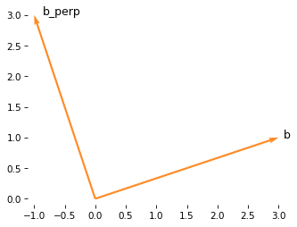
Here’s the vector perpendicular to b.
b_perp = vector_perpendicular(b)
b_perp
array([-1, 3])
And here’s what it looks like.
from utils import label_vector

plot_vector(b, color='C1', label='b')
plot_vector(b_perp, color='C1')
label_vector('b_perp', b_perp, label_pos=1, ha='left')
decorate_plane(xlim=[-1.1, 3.1], ylim=lim)
To confirm that they are perpendicular, we can compute the dot product.
b @ b_perp
0
The result is zero, which indicates that the vectors are perpendicular.
Now, we have everything we need for the pool example.
3.7. Collisions#
If you have ever played pool (or billiards) you are familiar with the behavior of rigid bodies when they collide. Billiard balls on a smooth table are often described with a simple physical model of elastic collision, developed by Christian Huygens in the 1600s.
But before we get to the physics, let’s set up the table. The playing surface of a tournament table has these dimensions in inches.
table_width = 100
table_height = 50
And standard pool balls have this diameter, also in inches.
ball_diameter = 2.25
As a first scenario, we’ll place the cue ball at the center of the left half of the table, and a target ball at the center of the right half. The following vectors represent these positions.
cue = np.array([25, 25])
target = np.array([75, 25])
Now we’ll create a vector that represents the velocity of the cue ball, 18 inches per second at an angle slightly above the \(x\) axis. We’ll specify it in polar coordinates and then convert to Cartesian.
v1 = pol2cart(r=16, phi=0.033)
v1
array([15.9913, 0.5279])
And let’s suppose the target ball is stationary, so its velocity is 0. We can come back and change it later.
v2 = pol2cart(r=0, phi=0)
v2
array([0., 0.])
After some time, t, we can compute the distance the balls have traveled relative to their starting places.
For example, here are the distances after 4 seconds.
t = 3
d1 = v1 * t
d2 = v2 * t
And we can compute the positions of the balls like this.
pos1 = cue + d1
pos2 = target + d2
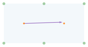
The following figure shows the table, the pockets, the positions of the two balls, and the distance traveled by the cue ball.
from utils import draw_table, draw_circles

draw_table()
plot_vector(d1, cue, color='C4')
draw_circles([cue, target])
[<matplotlib.patches.Circle at 0x7f21929b94b0>,
 <matplotlib.patches.Circle at 0x7f21929b95a0>]
Now let’s see how close the cue is to the target ball. We’ll use this function to compute the length of the difference between two vectors.
def distance_between(pos1, pos2):
    return norm(pos1 - pos2)
Here’s the final distance in this scenario.
distance_between(pos1, pos2)
2.5716
Here’s a zoomed in view showing the positions of the cue and target.
from utils import draw_collision

draw_collision(t, cue, target, v1, v2)
plot_vector(d1, cue, color='C4')
label_vector('d1', d1, cue, label_pos=11, va='bottom')
decorate_plane(xlim=[55, 95], ylim=[10, 40])
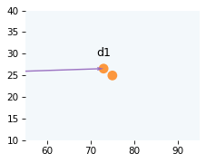
It looks as if the cue will hit the target if it keeps going in this direction. In the next section, we’ll check whether the balls will collide and figure out their positions when they do.
3.8. Collision Prediction#
To check whether the balls will collide, we’ll find the value of t that minimizes the distance between them.
Then we can check whether this distance is less than one diameter – if it is, they collide.
The following function takes a hypothetical value of t, the starting positions of the balls, and their velocities.
It returns the distance between the final position of the cue and the target.
def objective_func(t, start1, start2, v1, v2):
    pos1 = start1 + v1 * t
    pos2 = start2 + v2 * t
    return distance_between(pos1, pos2)
We can invoke the function directly.
objective_func(t, cue, target, v1, v2)
2.5716
But it is meant to be used with the minimize_scalar function, which searches for the value of t that minimizes the distance between the balls.
from scipy.optimize import minimize_scalar


def minimize_distance(start1, start2, v1, v2):
    args = (start1, start2, v1, v2)

    relative_speed = norm(v1 - v2)
    upper = distance_between(start1, start2) / relative_speed
    min_soln = minimize_scalar(
        objective_func, bounds=(0, upper), args=args, method="bounded"
    )

    assert min_soln.success
    return min_soln
To put an upper bound on the time until the collision, we compute the relative speed of the two balls, which is the length of the difference in velocities.
relative_speed = norm(v1 - v2)
relative_speed
16.0000
The time until the balls collide, if they do, can’t be longer than the initial distance between them divided by this speed.
Now here’s how we call minimize_distance.
min_soln = minimize_distance(cue, target, v1, v2)
The result is an OptimizeResult object that contains a message indicating whether the algorithm found a minimum within the bounds it searched.
min_soln.message
'Solution found.'
The x attribute contains the time that minimizes the distance.
t_min = min_soln.x
t_min
3.1233
And fun contains the objective function evaluated at x, which is the distance between balls.
min_soln.fun
1.6497
If this value is smaller than twice the radius (which is the diameter), that means the balls collide. We’ll use this function to check.
def will_hit(start1, start2, v1, v2, thresh):
    min_soln = minimize_distance(start1, start2, v1, v2)
    return min_soln.fun < thresh
With the initial direction we chose, the balls collide.
will_hit(cue, target, v1, v2, ball_diameter)
True
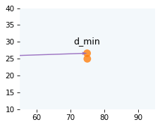
Here’s what it looks like when the distance between balls is minimized.
d_min = v1 * t_min
draw_collision(t_min, cue, target, v1, v2)
plot_vector(d_min, cue, color='C4')
label_vector('d_min', d_min, cue, label_pos=11, va='bottom')
decorate_plane(xlim=[55, 95], ylim=[10, 40])
The minimal distance tells us whether the balls will collide, but not when they will collide. For that, we have to do one more search.
3.9. Collision Detection#
To detect the instant the balls collide, we’ll search for the value if t where the distance between the balls is exactly one diameter, which means they are in contact.
The following function takes as arguments a hypothetical time in seconds, the starting positions of the balls, their velocities, and the distance between them we are searching for. It returns an error, which is the difference between the computed distance and the goal distance.
def error_func(t, start1, start2, v1, v2, goal_distance):
    actual_distance = objective_func(t, start1, start2, v1, v2)
    return actual_distance - goal_distance
For example, if we call it with the initial guess for t, we find that we are off by about a third of a second.
error_func(t, cue, target, v1, v2, ball_diameter)
0.3216
We can search more efficiently if we can provide a lower and upper bound on the solution.
As an upper bound, we’ll use t_min, which we know is too far.
For the lower bound, we’ll use 0 – we could provide a tighter bound, but it’s not necessary.
lower = 0
upper = t_min
Now we can use root_scalar to search for the value of t that makes the distance between balls exactly one diameter.
from scipy.optimize import root_scalar

args = (cue, target, v1, v2, ball_diameter)
root_soln = root_scalar(error_func, bracket=[lower, upper], args=args, method="brentq")
The result is a RootResults object that contains a flag that indicates whether the search converged to a solution.
root_soln.flag
'converged'
The root attribute contains the value of t at the instant of collision.
t_coll = root_soln.root
t_coll
3.0277
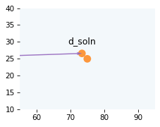
We can use to compute the offset vector.
d_soln = t_coll * v1
And here’s what it looks like at the instant of collision.
draw_collision(t_coll, cue, target, v1, v2)
plot_vector(d_soln, cue, color='C4')
label_vector('d_soln', d_soln, cue, label_pos=11, va='bottom')
decorate_plane(xlim=[55, 95], ylim=[10, 40])
Now let’s figure out what happens after the collision.
3.10. Elastic Collision#
In a perfectly elastic collision, total energy is conserved, but momentum is transferred from one body to another. In the real world, collisions are not perfectly elastic, but for rigid bodies like pool balls, it’s not a bad model.
When a ball with velocity \(v_1\) collides with another ball with velocity \(v_2\), we can figure out the velocities of both balls, after the collision, by following these steps.
Find a unit vector on the line of impact – that is, the line between the centers of the balls.
Compute the projection of both velocities onto this vector, and the rejection of both velocities, perpendicular to this vector.
If the balls have the same mass (which is close to true in tournament play), the components of the velocities along the center line are exchanged, and the perpendicular components are unaffected.
That’s the general idea – now let’s see the details. First, here are the positions of the balls at the point of impact.
pos1 = cue + v1 * t_coll
pos2 = target + v2 * t_coll
And here’s a unit vector on the line between the centers of the balls.
It’s called the normal vector because it’s perpendicular – in other words, normal to – the contact surface between the balls.
We’ll call it n_hat, where n stands for “normal” and hat indicates that it’s a unit vector.
from utils import normalize

n_hat = normalize(pos2 - pos1)
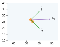
The perpendicular to the normal vector is called the tangent vector, which we’ll call t_hat.
t_hat = vector_perpendicular(n_hat)
The following figure shows the normal and tangent vectors (scaled so they are more visible).
draw_collision(t_coll, cue, target, v1, v2)
plot_vector(n_hat, pos1, label='$\hat{n}$', scale=10, color="C2")
plot_vector(t_hat, pos1, label='$\hat{t}$', scale=10, color="C2")
plot_vector(v1, pos1, label='$v_1$', color="C4")
decorate_plane(xlim=[55, 95], ylim=[10, 40])
Now we can compute the component of velocity in the direction of the normal vector, which is the projection of v1 on n_hat.
v1_normal = vector_projection(v1, n_hat)
And we have three ways to compute the component of velocity in the direction of the tangent vector.
We can compute the projection of v1 on t_hat.
v1_tangent = vector_projection(v1, t_hat)
v1_tangent
array([8.3334, 8.2568])
Or the rejection of v1 from n_hat.
v1_tangent = vector_rejection(v1, n_hat)
v1_tangent
array([8.3334, 8.2568])
Or, we can subtract from v1 its component in the direction of the normal vector, which we have already computed.
v1_tangent = v1 - v1_normal
v1_tangent
array([8.3334, 8.2568])
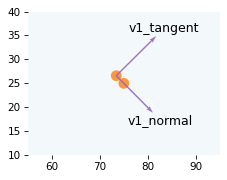
The following figure shows what those components look like.
draw_collision(t_coll, cue, target, v1, v2)
plot_vectors([v1_normal, v1_tangent], [pos1, pos1],
             labels=['v1_normal', 'v1_tangent'], color="C4")
decorate_plane(xlim=[55, 95], ylim=[10, 40])
Next we’ll split v2 into components the same way.
In this example, they are both zero, but we’ll come back and change that later.
v2_normal = vector_projection(v2, n_hat)
v2_tangent = v2 - v2_normal
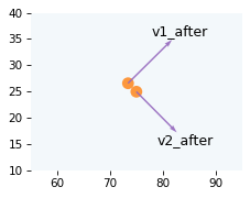
Finally, we can compute the velocities of both balls after the collision. In this example, because the masses are the same, the velocities along the tangent vector are unchanged and the velocities along the normal vector are exchanged.
v1_after = v1_tangent + v2_normal
v2_after = v2_tangent + v1_normal
Here’s what the velocities look like after the collision.
draw_collision(t_coll, cue, target, v1, v2)
plot_vectors([v1_after, v2_after], [pos1, pos2],
             labels=['v1_after', 'v2_after'], color="C4")
decorate_plane(xlim=[55, 95], ylim=[10, 40])
Now let’s see if the target ball goes in the pocket. Since we already have a way to check for collisions, we’ll create a virtual ball at the location of the pocket in the lower left corner – with velocity zero.
pocket2 = np.array([table_width, 0])
v_pocket = np.array([0, 0])
If the target ball hits the pocket ball, it would go in the pocket. In reality, that might be too generous. To simulate a tighter pocket, we could make the last argument smaller than the diameter of the ball. But let’s keep it simple.
will_hit(pos2, pocket2, v2_after, v_pocket, ball_diameter)
True
And it does! To see how close we are to the center of the pocket, we can compute the minimum distance between the target ball and the virtual ball.
min_soln = minimize_distance(pos2, pocket2, v2_after, v_pocket)
min_soln.fun
0.1633
It’s off by less than an inch, so that’s good!
But we have a problem. If the cue ball also goes in a pocket, the shot doesn’t count. So let’s check whether the cue ball hits the pocket in the upper right corner.
pocket1 = np.array([table_width, table_height])
will_hit(pos1, pocket1, v1_after, v_pocket, ball_diameter)
True
Oops.
As an exercise, go back and adjust the angle of v1 and see if you can find a value that puts the target ball in the pocket and keeps the cue ball on the table.
3.11. Animation#
If we’re going to simulate a physical system, it would be a shame not to animate the results.
First, let’s use root_scale one more time to find the time until the target ball hits the virtual ball that represents the pocket.
lower = 0
upper = min_soln.x

args = (pos2, pocket2, v2_after, v_pocket, ball_diameter)
root_soln = root_scalar(error_func, bracket=[lower, upper], args=args, method="brentq")
Here’s how long it takes.
t_sink = root_soln.root
t_sink
3.0432
Now let’s compute the total time, before and after the collision, and define equally spaced time steps between 0 and t_total.
dt is the number of milliseconds between time steps.
t_total = t_coll + t_sink
ts = np.linspace(0, t_total, 150)
dt = t_total / len(ts) * 1000
dt
40.4726
We’ll also compute the position of both balls at the instant of collision.
cue_coll = cue + t_coll * v1
target_coll = target + t_coll * v2
To animate the results, we’ll create (and then close) a figure that contains all of the objects at their starting positions.
fig, ax = draw_table()
plot_vector(v1, cue, color='C4')
quiver = plot_vectors([v1_after, v2_after], [cue_coll, target_coll], color='C4')
quiver.set_visible(False)

cue_patch, target_patch = draw_circles([cue, target])
plt.close(fig)
The animate function takes a frame number, looks up the corresponding time step, t, and moves the objects to their positions at t.
def animate_frame(frame_num):
    t = ts[frame_num]

    if t < t_coll:
        pos1 = cue + t * v1
        pos2 = target + t * v2
    else:
        t2 = t - t_coll
        pos1 = cue_coll + t2 * v1_after
        pos2 = target_coll + t2 * v2_after
        quiver.set_visible(True)

    cue_patch.center = pos1
    target_patch.center = pos2

    return cue_patch, target_patch
Finally, we can make the animation.
import matplotlib.animation as animation

anim = animation.FuncAnimation(
    fig,
    animate_frame,
    frames=len(ts),
    interval=dt,
)
And display it.
from IPython.display import HTML

HTML(anim.to_jshtml())
3.12. Exercises#
3.12.1. Exercise#
On some coin-operated pool tables, the cue ball is heavier than the target balls, which makes it easier for the ball return mechanism to separate out the cue ball. But some players find that this difference affects the behavior of the balls. Let’s see how much.
In the general case, where the masses of the two balls are \(m_1\) and \(m_2\), here’s how we can compute the velocities of the balls after the collision, \(v_1'\) and \( v_2'\):
where \(\operatorname{proj}_{\hat{n}}(v_1 - v_2)\) is the vector projection of the relative velocity on n_hat.
Suppose the target ball is 6 ounces (168 g) and the cue ball is 6.7 ounces (188 g). Compute the velocities of the balls after the collision and check to see whether the target still hits the pocket. Also compute the minimum distance between the target ball and the virtual ball in the pocket, and the time it takes to get there.
What difference does it make when the weights are different?
Hint: Check your solution by testing it with equal weights.
3.12.2. Exercise#
In pool it is not legal to take a shot while any of the balls on the table are still moving, but just for fun, go back and set v2 to a non-zero velocity, and see if you can find a value of v1 that pockets the target ball.
Copyright 2025 Allen B. Downey
Code license: MIT License
Text license: Creative Commons Attribution-NonCommercial-ShareAlike 4.0 International