Think Linear Algebra is not for sale yet, but if you would like to support this project, you can buy me a coffee.
4. To Boldly Go#
When I was an undergraduate, I took a mini-course on computer graphics. I remember one (and only one) of the assignments, partly because it took me a long time to get it working, and partly because it was so satisfying when I did. It was about affine transforms and image processing, and the image we used was a line drawing of the starship Enterprise from Star Trek.
In this chapter, we’ll replicate this assignment and boldly go beyond it. We’ll start with image processing, using a photo of the Enterprise – that is, the model used to make the television show – to create an outline of the ship as a collection of vectors.
We’ll use array operations to implement transformations like flipping, shifting and scaling. Then we’ll do the same operations using matrix multiplication, which makes it possible to compose multiple transformations into a single step.
As a next step, we’ll use homogeneous coordinates to implement affine transformations, which makes it possible to translate vectors – that is, shift them in space.
To simulate a starship orbiting a planet, we’ll do some physics, using an ODE solver to compute the orbit, and testing Kepler’s second law.
Finally, we’ll bring it all together to generate an animation of the ship revolving around the planet while rotating and changing shape.
There’s a lot in this chapter, but if you persist, I hope you’ll enjoy it as much as I did.
Click here to run this notebook on Colab.
Show code cell content
from os.path import basename, exists


def download(url, filename=None):
    if filename is None:
        filename = basename(url)

    if not exists(filename):
        from urllib.request import urlretrieve

        local, _ = urlretrieve(url, filename)
        print("Downloaded " + local)


download("https://github.com/AllenDowney/ThinkLinearAlgebra/raw/main/utils.py")
Show code cell content
import networkx as nx
import numpy as np
import pandas as pd
import matplotlib.pyplot as plt
import sympy as sp

from utils import decorate, underride
4.1. Image Processing#
If you have worked with computer graphics, you might know that there are two common ways to represent images, bitmaps and vectors. A bitmap is like an array where each element represents the color of a pixel. A vector represents a coordinate in space.
If you have an image in vector format, you can create a bitmap by rendering the vectors. If you have an image in bitmap format, it is not as easy to generate vectors, but there are image processing algorithms that make it possible.
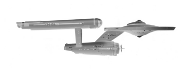
As an example, we’ll start with an image of the starship Enterprise from the original series of Star Trek. The model used in the television show is now in the Smithsonian National Air and Space Museum. The following cell downloads a photo of the model, originally from the museum’s web site.
filename = "NASM-A19740668000-NASM2016-02687-000001-scaled.jpg"

download(f"https://github.com/AllenDowney/ThinkLinearAlgebra/raw/main/data/{filename}")
scikit-image provides functions we’ll use to process the image, starting with io.imread, which reads the image and returns a NumPy array.
from skimage import io, color, filters, measure

image = io.imread(filename)
image.shape
(287, 750, 3)
The array has 750 columns and 287 rows of pixels, and each pixel is represented by three numbers that represent levels of red, green, and blue (RGB).
We’ll use color.rgb2gray to convert the image from RGB to grayscale.
gray = color.rgb2gray(image)
gray.shape
(287, 750)
The result is a NumPy array with one number per pixel, in the range from 0, which represents black, to 1, which represents white.
We can use the Matplotlib function imshow to display the image.
The color map gray_r reverses the scale, showing the image in negative – so it appears in shades of gray on a white background.
plt.imshow(gray, cmap="gray_r")
plt.axis("off");
scikit-image provides find_contours, which takes an image and finds a sequence of line segments that trace the boundary between light and dark regions.
The level parameter is the threshold that determines how dark is considered dark.
contours = measure.find_contours(gray, level=0.05)
len(contours)
10
The result is a list of contours – each of them is a NumPy array with one row for each point that makes up the contour. We’ll select the first array in the list, which represents the perimeter of the ship.
contour = contours[0]
contour.shape
(2493, 2)
The array has 2493 rows, one for each point, and two columns, containing the coordinates of a pixel in the image.
We’ll use the T attribute to transpose the array.
The result has two rows containing the y and x coordinates of the pixels – in that order – which we can assign to separate variables.
ys, xs = contour.T
It will be efficient to reduce the number of points in the contour.
For that, we’ll use a LineString object and its simplify method.
from shapely.geometry import LineString

line = LineString(np.transpose([xs, ys]))
simplified = line.simplify(tolerance=2.5)
The result is a LineString object that approximates the contour with fewer points.
The tolerance argument determines how close the approximation is.
We can select coords from the result and convert to a NumPy array.
coords = np.array(simplified.coords)
coords.shape
(59, 2)
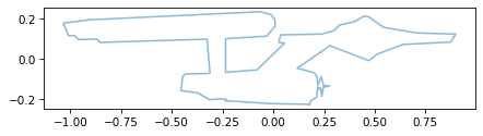
The result has only 59 points, which is much more manageable. We’ll use the following function to plot contours.
def plot_contour(contour, **options):
    underride(options, color="C0", alpha=0.5)
    rows, cols = contour.shape
    if rows not in [2, 3]:
        contour = contour.T

    xs, ys = np.array(contour)[:2]
    plt.plot(xs, ys, **options)
    decorate(aspect='equal')
This function is very forgiving – it works if the array has either two or three rows, or if it has two or three columns. This flexibility will be convenient later when we represent contours in different formats.
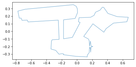
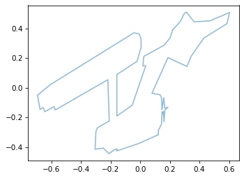
Here’s what the contour looks like.
plot_contour(coords)
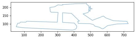
The result looks good, but you might notice that it is upside down.
That’s because find_contour uses image coordinates, where the y axis points down, and Matplotlib uses Cartesian coordinates, where the y axis points up.
In the next section, we’ll flip it.
4.2. Transformations#
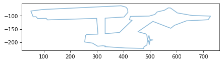
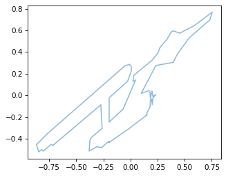
To flip the y coordinates and leave the x coordinates alone, we can multiply coords by the list [1, -1].
flipped = coords * [1, -1]
plot_contour(flipped)
Let’s unpack how that works.
Because coords is an array, the list gets converted to an array with shape (2,) – that is, one dimension with length 2.
array = np.array([1, -1])
array.shape
(2,)
The shape of coords is (67, 2), which we can think of as 67 rows and 2 columns.
coords.shape
(59, 2)
Because the last element of the shapes is the same, array can be broadcast to have the same shape as coords.
We can do the broadcast explicitly like this.
broadcast = array[None, :]
broadcast.shape
(1, 2)
None represents a new dimension, and : selects all elements of the existing dimension.
The result has shape (1, 2), which we can think of as one row and two columns.
Then when we multiply by coords, the row gets copied 67 times.
flipped = coords * broadcast
flipped.shape
(59, 2)
So the result has the same shape as coords.
We can use a similar pattern to shift the coordinates so the center of the ship is at the origin.
First we’ll compute the mean of the coordinates along the first axis.
The argument axis=0 means that the first axis is eliminated, leaving only the second, with length 2.
mean = flipped.mean(axis=0)
mean
array([ 413.23 , -144.215])
The result is the mean of the rows.
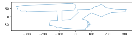
If we subtract it from flipped, it gets broadcast and subtracted from each row – so each coordinate gets shifted left by about 413 pixels and up by about 141.
shifted = flipped - mean
The result looks the same, but now it’s centered at the origin.
plot_contour(shifted)
While we’re at it, let’s scale the coordinates down so the largest coordinate is about 1.
For that we don’t need an array – we can divide all of the elements by a scalar.
scaled = shifted / 350
plot_contour(scaled)
The operations we performed in this section – flip, shift, and scale – are examples of transformations. We performed them using array operations, but they can also be expressed using vector and matrix operations, as we’ll see soon.
But first let’s consider two ways to represent vectors.
4.3. Row Vectors and Column Vectors#
In the examples so far, we’ve used NumPy arrays with one row for each vector, and two columns. For example, the simplified contour of the ship has 59 rows, one for each point on the contour.
coords.shape
(59, 2)
Vectors in this form are called row vectors. This form works well with NumPy because we can iterate through the vectors by iterating through the rows of the array. And we can shift and scale the vectors using array operators like addition and multiplication.
An alternative is to transpose the array so it has two rows and one column per vector.
transposed = coords.T
transposed.shape
(2, 59)
Vectors in this form are called column vectors.
This format is convenient if we want to extract the coordinates of the points as separate arrays, as we do in plot_contour.
xs, ys = transposed
xs.shape
(59,)
This format is also useful when we perform linear algebra operations like matrix multiplication. As we’ll see in the next few sections, most linear algebra operations are defined in terms of column vectors, and don’t work with row vectors.
Before we go on, let’s save the shifted, scaled version of the contour.
ship = scaled
ship.shape
(59, 2)
Now let’s do some linear algebra.
4.4. Contours and Vectors#
So far we’ve been thinking of ship as a sequence of coordinate pairs.
To plot it, we can separate the x and y coordinates and use Matplotlib to connect the dots.
xs, ys = ship.T
plt.plot(xs, ys, ".-", alpha=0.3)
decorate(aspect='equal')
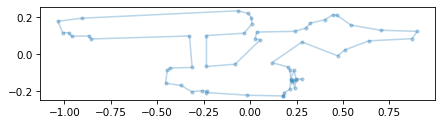
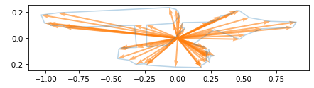
But we can also think of ship as a collection of vectors with their tails at the origin and their heads on the contour.
We can use plot_vectors to see what that looks like.
from utils import plot_vectors

plt.plot(xs, ys, "-", alpha=0.3)
plot_vectors(ship, width=0.005, color="C1")
decorate(aspect='equal')
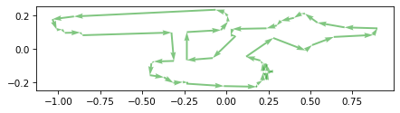
Now to connect the dots, we can use vector subtraction to compute the difference between each vector and the next.
rolled = np.roll(ship, shift=1, axis=0)
diffs = rolled - ship
To see how that works, let’s consider the first three rows of ship.
ship[:3]
array([[ 0.179, -0.224],
       [-0.015, -0.221],
       [-0.238, -0.206]])
And the first three rows of rolled.
rolled[:3]
array([[ 0.179, -0.224],
       [ 0.179, -0.224],
       [-0.015, -0.221]])
rolled contains the coordinate pairs from ship, with each one shifted down one position, and the last rolled around to become the first.
When we subtract, the result contains vectors that connect each point on the contour to the next – which we can plot like this.
plot_vectors(diffs, ship, width=0.005, color="C2")
decorate(aspect='equal')
If we think of coordinates as vectors, we can think of transformations like shifting and scaling as vector operations – and that turns out to be useful. Let’s start with scaling.
4.5. Scale#
In this section we’ll represent scaling as a vector-matrix product. To show what that means, we’ll use this function to make a column vector.
def make_vector(x, y):
    return np.array([[x], [y]])
As an example, we’ll create a vector with symbolic coordinates x and y.
from sympy import symbols

x, y = symbols('x y')
v = make_vector(x, y)
To display vectors and matrices, we’ll use the SymPy Matrix class.
from sympy import Matrix

Matrix(v)
Now we’ll use the following function to make a scale matrix.
The parameters sx and sy specify the scale factor in the x and y directions.
def scale_matrix(sx, sy):
    return np.array([[sx, 0], [0, sy]])
To show what that looks like, I’ll create a scale matrix with symbolic values of sx and sy.
sx, sy = symbols('s_x s_y')

S = scale_matrix(sx, sy)
Matrix(S)
Now we can multiply S and v using the matrix multiplication operator, @.
Matrix(S @ v)
The result is a column vector where the x coordinate has been multiplied by sx and the y coordinate has been multiplied by sy.
To make the example more concrete, I’ll make a matrix that compresses the x coordinate by 25% and stretches the y coordinate by 50%.
S = scale_matrix(0.75, 1.5)
Matrix(S)
Now let’s apply this transformation to the contour of the ship. Because the contour is a collection of row vectors, and the matrix requires column vectors, we have to transpose the contour before applying the transformation.
scaled = S @ ship.T
scaled.shape
(2, 59)
The result is a collection of column vectors. Here’s what it looks like.
plot_contour(scaled)
As expected, it is compressed in the x direction and stretched in the y direction.
Now let’s consider two other transformations, shear and rotation.
4.6. Shear#
Shearing is a transformation it will be easier to show than describe.
We’ll start by making a shear matrix that takes two parameters, the amount of shear in the x and y directions.
def shear_matrix(kx, ky):
    return np.array([[1, kx],
                     [ky, 1]])
Here’s what it looks like with symbolic elements.
kx, ky = symbols('k_x, k_y')

K = shear_matrix(kx, ky)
Matrix(K)
And here’s the effect it has if we multiply by a vector.
Matrix(K @ v)
The shear matrix adds some fraction of y to the x coordinate and some fraction of x to the y coordinate.
But it’s probably still not clear what that means.
As an example, we’ll make a matrix that represents a horizontal shear with kx = 0.5.
K = shear_matrix(0.5, 0)
Matrix(K)
Here’s the effect on a symbolic vector.
Matrix(K @ v)
Every point gets shifted to the right by half of its y coordinate.
Let’s see what that looks like if we apply it to the ship.
sheared = K @ ship.T
It will be easier to see the result if we make a bounding box.
from matplotlib.transforms import Bbox

def make_bbox(contours):
    """Makes the bounding box of a list of contours."""
    box = Bbox.null()
    for contour in contours:
        box.update_from_data_xy(contour, ignore=False)

    index = [0, 1, 3, 2, 0]
    return box.corners()[index]
And apply the same transform to the bounding box.
bbox = make_bbox([ship])
bbox_sheared = K @ bbox.T
plot_contour(sheared)
plot_contour(bbox_sheared, color='C1')
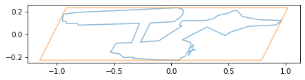
If we think of the bounding box as a stack of sheets of paper, a horizontal shear has the effect of shifting the sheets to the right in proportion to their height.
As an exercise at the end of the chapter, you’ll have a chance to experiment with a vertical shear and the composition of a horizontal and vertical shear.
4.7. Rotation#
In addition to scaling and shearing, we can also express rotation using matrix multiplication. We’ll start by defining a unit vector that specifies the angle of rotation.
from utils import normalize

v_hat = normalize([1, 0.5])
Along with v_hat, we’ll also need a perpendicular vector we’ll call v_perp.
def vector_perp(v):
    x, y = v
    return np.array([-y, x])
v_perp = vector_perp(v_hat)
Here’s what those vectors look like, along with unit vectors that represent the x and y axes.
i_hat = np.array([1, 0])
j_hat = np.array([0, 1])
plot_vectors([i_hat, j_hat],
             labels=['i_hat', 'j_hat'], label_pos=[11, 1])
plot_vectors([v_hat, v_perp], color='C1',
             labels=['v_hat', 'v_perp'], label_pos=[11, 1])
decorate(aspect='equal')
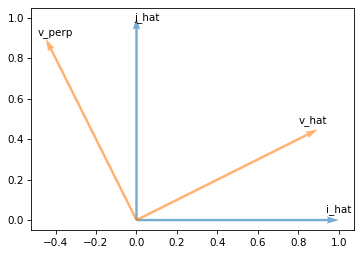
This rotation transforms i_hat axis to v_hat and j_hat axis to v_perp.
So one way to specify a rotation is by building a matrix with v_hat and v_perp as columns – which we can do most conveniently by stacking them as rows and then transposing.
def rotation_matrix(v_hat):
    v_perp = vector_perp(v_hat)
    return np.array([v_hat, v_perp]).T
Here’s an example based on v_hat.
R = rotation_matrix(v_hat)
Matrix(R)
Now if we multiply by the x axis, it selects the first column of the matrix, which is v_hat.
Matrix(R @ i_hat.T)
If we multiply by the y axis, it selects the second column of the matrix, which is v_perp.
Matrix(R @ j_hat.T)
And if we multiply by any other vector, the effect is to rotate the vector by the same amount we rotated the axes. As an example, we’ll rotate the vectors in the contour of the ship.
rotated = R @ ship.T
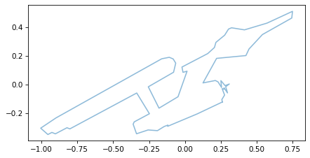
The effect is to rotate the ship around the origin.
plot_contour(rotated)
At this point we’ve created matrices that scale, shear, and rotate vectors. Now let’s put them together!
4.8. Composition#
Here are the scaled, shifted, and rotated versions of the ship, all in one place.
scaled = S @ ship.T
sheared = K @ ship.T
rotated = R @ ship.T
If we want to apply all three transforms, we can compose them like this:
transformed = R @ K @ S @ ship.T
plot_contour(transformed)
We can think of that calculation as three matrix-vector multiplications, like this:
transformed1 = R @ (K @ (S @ ship.T))
Or we can think of it as two matrix-matrix multiplications, followed by a matrix-vector multiplication.
M = R @ K @ S
transformed2 = M @ ship.T
M is a transformation matrix that performs all three operations: scaling, shearing, and rotating, in a single step.
Matrix(M)
plot_contour(transformed2)
But the order of the operations matters. If we perform the operations in the opposite order, we get a different transformation matrix.
M2 = S @ K @ R
Matrix(M2)
And the effect is visibly different.
reverse_order = M2 @ ship.T

plot_contour(reverse_order)
So we can express any combination of scaling, shearing, and rotation with a single matrix.
Now let’s consider one more operation: moving or shifting the contour, more formally known as translation.
4.9. Translation#
To move the ship in space, we can use array addition, as we did in Section xxx.
shifted = ship + [1, 0.5]
plot_contour(ship)
plot_contour(shifted, color='C1')
Unfortunately, there is no way to represent this operation as matrix multiplication – at least, not with a 2x2 matrix. But with a 3x3 matrix, we can do it!
We’ll use this function to create a translation matrix that adds dx to the x coordinate and dyto the y coordinate.
def translation_matrix(dx, dy):
    return np.array([[1, 0, dx],
                     [0, 1, dy],
                     [0, 0, 1]])
To show how it works, we’ll make a matrix with symbolic values of dx and dy.
dx, dy = symbols('dx dy')

T = translation_matrix(dx, dy)
Matrix(T)
This matrix doesn’t work with a standard two-dimensional vector.
We have to make a three-dimensional vector that contains x, y, and an third coordinate, which we’ll set to 1.
x, y = symbols('x y')
v3 = np.array([[x], [y], [1]])
Matrix(v3)
This way of representing a vector is called homogeneous coordinates. Now if we compute the matrix-vector product, we can see the effect.
Matrix(T @ v3)
The x and y coordinates are shifted by dx and dy, and the third coordinate is preserved.
Now let’s apply this transformation to the contour of the ship.
Remember that ship contains 59 row vectors.
ship.shape
(59, 2)
We can augment it by adding a third column of ones.
def augment_contour(contour):
    rows, cols = contour.shape
    ones = np.ones((rows, 1))
    return np.hstack([contour, ones])
The result has 59 rows and three columns.
ship3 = augment_contour(ship)
ship3.shape
(59, 3)
Let’s make a translation matrix that shifts one unit to the right and a half unit up.
T = translation_matrix(1, 0.5)
Now we can move the ship.
translated = T @ ship3.T
translated.shape
(3, 59)
The result contains 3 rows, one for each coordinate, and 59 columns.
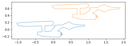
We can use plot_contour to see the results.
plot_contour(ship)
plot_contour(translated, color='C1')
Now that we can express translation as matrix multiplication, we can combine it with the other operations, as we’ll demonstrate in the next example.
4.10. Ellipse#
As an example that combines translation and scaling, let’s make an ellipse. First we’ll create an array of angles from 0 to \(2 \pi\).
n = 100
thetas = np.linspace(0, 2 * np.pi, n)
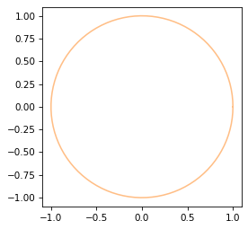
We can use cos and sin to compute the x and y coordinates of points on a circle with radius 1.
xs = np.cos(thetas)
ys = np.sin(thetas)
Then we’ll pack the results into a contour.
circle = np.transpose([xs, ys])
circle.shape
(100, 2)
We can plot it like this.
plot_contour(circle, color='C1')
To make it an ellipse, we’ll scale it by a and b, which are the lengths of the semi-major and semi-minor axes.
a, b = 6, 5

S = scale_matrix(a, b)
Matrix(S)
And we’ll shift it by c, which is the distance from the center of the ellipse to the focus.
c = np.sqrt(a**2 - b**2)
T3 = translation_matrix(c, 0)
Matrix(T3)
Before we can apply the translation, we have to augment the circle with a third coordinate.
circle3 = augment_contour(circle)
circle3.shape
(100, 3)
Similarly before we can combine the transformations, we have to augment the scaling matrix with an additional row and column.
def augment_matrix(M):
    """Augment a 2x2 matrix into a 3x3 homogeneous transform."""
    H = np.eye(3)
    H[:2, :2] = M
    return H
Here is the augmented version of the scaling matrix.
S3 = augment_matrix(S)
Matrix(S3)
Now we can combine the transforms.
M = T3 @ S3
Matrix(M)
And apply them to the circle.
ellipse3 = M @ circle3.T

plt.plot(0, 0, '.')
plot_contour(ellipse3)
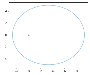
Using homogeneous coordinates makes it possible to compose translation with the other transforms: scale, shear, and rotation.
4.11. Orbit#
Now let’s bring it all together and replicate the exercise I worked on as an undergraduate: drawing a starship orbiting a planet. To make it a little more interesting, we’ll use an ODE solver to compute the position and velocity of an object in orbit, due to the force of gravity. If you are not familiar with ordinary differential equations (ODEs), you don’t have to understand all of the details.
To solve a differential equation numerically, we need a function that computes derivatives. For this problem, specifically, this function takes the position and velocity of the orbiting object at a particular point in time, and it computes the acceleration of the object.
As an example, we’ll start with the object at position (7, 0) with velocity (0, 5). The units of length and time have been scaled so all the numbers are small in magnitude. Here’s a list of values that represent the initial conditions in the format required by the ODE solver.
x0 = 7.0
y0 = 0.0
vx0 = 0.0
vy0 = 5.0

init = [x0, y0, vx0, vy0]
Now we’ll compute the derivative of the initial condition, which is the acceleration of the object due to gravity. We’ll start by packing the position and velocity into vectors.
r_vec = [x0, y0]
v_vec = [vx0, vy0]
By the law of universal gravitation, the magnitude of the acceleration is \(\mu / r^2\) – where \(\mu\) is a constant that depends on the mass of the planet and \(r\) is the distance of the object from the planet – and the direction of acceleration is toward the planet. So we can compute an acceleration vector like this.
from utils import norm

mu = 400
r = norm(r_vec)
r_hat = r_vec / r
a_vec = -mu / r**2 * r_hat
a_vec
array([-8.163, -0. ])
r is the length of the position vector, which is the distance of the object from the planet.
r_hat is a unit vector that points from the planet to the object, so when it’s negated, it points from the object to the planet.
The following function encapsulates these steps and provides the interface required to work with the ODE solver.
Specifically, it takes as parameters time, t, and a state vector, u, that contains the coordinates of position and velocity.
It returns the derivative of the state vector, du/dt, which contains the coordinates of velocity and acceleration.
from utils import norm

def deriv_func(t, u):
    """
    Compute time derivatives for state u = [x, y, vx, vy]

    Returns du/dt = [vx, vy, ax, ay]
    """
    x, y, vx, vy = u

    r_vec = [x, y]
    v_vec = [vx, vy]

    r = norm(r_vec)
    r_hat = r_vec / r
    a_vec = -mu / r**2 * r_hat

    return np.hstack([v_vec, a_vec])
Before we call the ODE solver, we have to specify a span of time to simulate. I’ve chosen a value that spans one complete orbit, approximately.
t_span = (0, 2.96)
t_span
(0, 2.960)
And we’ll specify that we want the solution to be evaluated at 100 equally spaced points in time.
t_eval = np.linspace(t_span[0], t_span[1], 100)
Here’s how we call the ODE solver.
rtol specifies the precision of the solution – in this case we need more precision than normal so the orbit returns to where it started, approximately.
from scipy.integrate import solve_ivp

solution = solve_ivp(deriv_func, t_span, init, t_eval=t_eval, rtol=1e-5)
The result is an object that contains information about the solution, including an array, y, that contains the coordinates of position and velocity.
solution.y.shape
(4, 100)
We’ll extract the first two columns, which we think of as a collection of position vectors, and the last two columns, which we think of as a collection of velocity vectors.
orbit = solution.y[:2].T
velocity = solution.y[2:, :].T
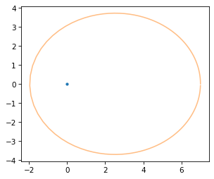
Here’s what the resulting orbit looks like with a dot indicating the location of the planet.
plt.plot(0, 0, '.')
plot_contour(orbit, color='C1')
As an example, let’s examine the position vector with index 20.
index = 20
r_vec = orbit[index]
r_vec
array([5.504, 2.762])
And the corresponding velocity vector.
v_vec = velocity[index]
v_vec
array([-5.126, 3.786])
Here’s what they look like, plotted along with the orbit.
from utils import plot_vector

plt.plot(0, 0, '.')
plot_vector(r_vec, label='r', label_pos=2, color='C2')
plot_vector(v_vec, r_vec, scale=0.4, label='v', label_pos=10)
plot_contour(orbit, color='C1')
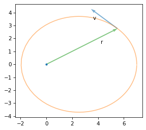
r is the vector from the planet to the ship and v is the velocity of the ship when it’s at that position.
I’ve scaled v to fit the diagram.
4.12. Transforming the Ship#
Given the position and velocity of the ship and a point in time, we’ll perform the following transformations, in this order.
Flip the ship vertically so the ventral side (belly) faces the planet.
Scale the ship horizontally so it’s longer when it’s going faster.
Rotate the ship so its axis is aligned with its velocity.
Translate the ship to its position relative to the planet.
Here’s the first transform, an augmented scale matrix that flips the ship vertically.
F3 = augment_matrix(scale_matrix(1, -1))
Matrix(F3)
The second transform stretches the ship, using an equation similar to the Lorenz factor that appears in special relativity, but with the sign changed so the ship gets longer when it’s going faster, rather than shorter (because on TV it’s better to look cool than be scientifically accurate).
v = norm(v_vec)
speed_of_light = 20
sx = np.sqrt(0.4 + v / speed_of_light)
sx
0.848
Here’s the augmented scaling matrix.
S3 = augment_matrix(scale_matrix(sx, 1))
Matrix(S3)
Here’s the rotation matrix that aligns the axis of the ship with its velocity.
v_hat = v_vec / v
R3 = augment_matrix(rotation_matrix(v_hat))
Matrix(R3)
And the translation matrix that moves it from the origin to its position.
T3 = translation_matrix(*r_vec)
Matrix(T3)
We can combine the transforms into a single matrix.
M3 = T3 @ R3 @ S3 @ F3
And apply it to the ship, like this:
transformed = M3 @ ship3.T
Here’s what it looks like after all that.
plt.plot(0, 0, '.')
plot_contour(orbit, color='C1')
plot_vector(r_vec, color='C2')
plot_contour(transformed)
Now let’s animate it.
4.13. Animation#
The following function encapsulates the steps from the previous section. As parameters it takes position and velocity vectors; it returns a transformation matrix.
def compute_transform(r_vec, v_vec, speed_of_light=20):
    F3 = augment_matrix(scale_matrix(1, -1))

    v = norm(v_vec)
    sx = np.sqrt(0.4 + v / speed_of_light)
    S3 = augment_matrix(scale_matrix(sx, 1))

    v_hat = v_vec / v
    R3 = augment_matrix(rotation_matrix(v_hat))

    T3 = translation_matrix(*r_vec)

    return T3 @ R3 @ S3 @ F3
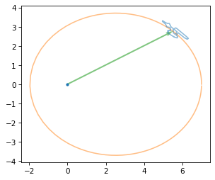
The following figure shows the ship at equally spaced points in its orbit.
plt.plot(0, 0, '.')
plot_contour(orbit, color='C1')

for r_vec, v_vec in zip(orbit[::10], velocity[::10]):
    M3 = compute_transform(r_vec, v_vec)
    transformed = M3 @ ship3.T
    plot_contour(transformed)
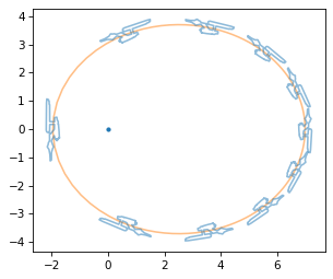
The length of the ship and the distance between steps indicate that the ship moves faster on the left when it is closer to the planet, and slower on the right when it is farther away.
In fact, we can use these results to check Kepler’s Second Law, that the orbit sweeps out an equal area in equal time.
First we’ll compute the distance the object travels in a short time, dt.
dt = 0.2
dr_vec = dt * v_vec
The area swept in this time is half of the the parallelogram spanned by r_vec and dr_vec, as shown in this diagram.
from utils import plot_vector

plt.plot(0, 0, '.')
plot_vector(r_vec, label='$r$', label_pos=2, color='C2')
plot_vector(dr_vec, color='C2')

plot_vector(r_vec, dr_vec)
plot_vector(dr_vec, r_vec, label='$dr$', label_pos=3)

diag = r_vec + dr_vec
xs = [0, r_vec[0], diag[0]]
ys = [0, r_vec[1], diag[1]]
plt.fill(xs, ys, alpha=0.3, color="gray")

plot_contour(orbit, color='C1')
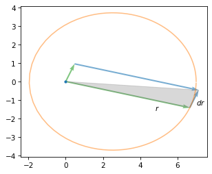
The area of that parallelogram is the cross product of the vectors, so we can use cross2d to compute the area of the shaded triangle.
from utils import cross2d

area = cross2d(r_vec, dr_vec) / 2
area
3.500
If we compute the cross product of corresponding vectors from orbit and velocity * 2, the result is an array of products.
areas = cross2d(orbit, velocity * dt) / 2
np.mean(areas)
3.500
Their mean is close to the area we just computed for a particular case. And the standard deviation is very small, which implies that the values are almost all the same.
np.std(areas)
0.000
This confirms Kepler’s law, and provides insight into why it holds. If we multiply the cross product of position and velocity by the mass of the object, the result is its angular momentum. So as long as the mass of the object doesn’t change, Kepler’s law is equivalent to conservation of angular momentum.
Now let’s make the animation.
The following function draws one frame.
It uses frame_num as an index into the orbit and velocity contours, transforms the ship to the right scale, orientation, and location, and uses the result to modify the coordinates of the ship_line object (defined below).
def animate_frame(frame_num):
    r_vec = orbit[frame_num]
    v_vec = velocity[frame_num]
    M3 = compute_transform(r_vec, v_vec)
    transformed = M3 @ ship3.T
    coords = transformed[:2, :]
    ship_line.set_data(*coords)
Before we start the animation, we create a figure that shows the planet, the orbit and the ship – but the coordinates of the ship are initially empty.
import matplotlib.animation as animation

fig, ax = plt.subplots()
plt.plot(0, 0, '.')
[orbit_line] = plt.plot(*orbit.T, alpha=0.5, color="C1")
[ship_line] = plt.plot([], [], alpha=0.5, color="C0")
ax.set_aspect('equal')

anim = animation.FuncAnimation(fig,
                               animate_frame,
                               frames=len(orbit),
                               interval=50)

plt.close(fig)
When we call FuncAnimation, the result is an object with all the information needed to create the animation.
The to_jshtml method calls animate_frame at each position in the orbit, generates a sequence of frames, and returns a JavaScript-driven HTML animation.
from IPython.display import HTML

HTML(anim.to_jshtml())
Press the play button – and I hope you are as entertained as I was, in 1987, by a much simpler version of this exercise.
4.14. Discussion#
Matrices actually better? Flip, scale, and shift are easier with array operations.
Linear and affine transformations
Any combination of affine transformations can be expressed with a matrix.
Any matrix can be decomposed into a combination of affine transformations, but not uniquely: there can be many combinations of transforms that yield the same matrix.
4.15. Exercises#
Flipping (reflection) as a special case of scaling
Projection as a special case of rotation and scaling
Rotate the ellipse around its focus
4.15.1. Shear and Italics#
If you are getting tired of transforming the Enterprise, let’s try something different. The following function takes a line of text, a font name, and a size, and returns a list of contours that render the text.
from matplotlib.textpath import TextPath
from matplotlib import font_manager

def get_text_contours(text, font="DejaVu Sans", size=100):
    font_path = font_manager.findfont(font)
    font_prop = font_manager.FontProperties(fname=font_path)
    tp = TextPath((0, 0), text, size=size, prop=font_prop)
    return tp.to_polygons()
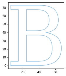
Here’s an example that creates contours for the letter B.
contours = get_text_contours("B", font="DejaVu Serif")
len(contours)
3
There are three contours, one for the outline and two for the holes. Here’s how we can plot them.
for contour in contours:
    plot_contour(contour)
One way to generate italic letter is to use a shear transform. Create a shear matrix, apply it to the contours, and plot the results. Try it with a string that contains a variety of letter and choose a shear parameter that gives the letters an aesthetically pleasing slant.
4.16. Asteroids#
Asteroids was a coin-operated arcade game released in 1979 by Atari.
It used vector graphics to draw a spaceship, flying saucers, and a collection of jagged-shaped asteroids.
The object of the game was to shoot the asteroids while avoiding collisions.
Here’s a video that shows what the game looked like.
With the limited computing power of the time, the graphics had to be generated as efficiently as possible.
Although the asteroids looked random, there were only four patterns – each could be drawn at three different sizes.
The code for the original game is available from 6502disassembly.com (6502 is the name of the processor the game ran on).
It includes the asteroid shapes as a sequence of SVEC commands, which could be interpreted by Atari’s Digital Vector Generator (DVG).
Each SVEC is a line segment, so a sequence of SVECs is a contour.
As an example, here’s the representation of the first asteroid shape.
svec_asteroid1 = [
    [ 0,  1,  1, -1,  1, -3, -3, -1,  0,  1,  1],  # dx
    [ 1,  1, -1, -2, -2, -2,  0,  1,  2,  1, -1],  # dy
    [ 3,  3,  3,  2,  2,  2,  2,  3,  3,  3,  3]   # scale
]
The first two rows contain offsets in the x and y directions.
The third row controls the size of the vectors.
The following function takes an array in this format and converts it to an array of x and y coordinates.
def make_contour_from_svec(svec):
    svec = np.asarray(svec)
    scale = svec[2]
    steps = svec[:2] * 2 ** scale
    contour = np.cumsum(steps, axis=1)
    return contour
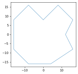
Here’s how we can convert and plot the first asteroid shape.
contour = make_contour_from_svec(svec_asteroid1)
plot_contour(contour)
And here are the other three asteroid shapes.
svec_asteroid2 = [
    [ 2,  2, -1, -2, -2, -1,  1, -1,  1,  1,  3,  2, -1],
    [ 1,  1,  1, -1,  1, -1, -2, -2, -1,  1, -1,  3,  1],
    [ 2,  2,  3,  2,  2,  3,  2,  2,  3,  2,  2,  2,  3],
]

svec_asteroid3 = [
    [-1, -2,  2,  2,  0,  1,  2,  0, -2, -3, -3,  2],
    [ 0, -1, -3,  3, -3,  0,  3,  1,  3,  0, -3, -1],
    [ 3,  2,  2,  2,  2,  3,  2,  3,  2,  2,  2,  2],
]

svec_asteroid4 = [
    [ 1,  3,  0, -3, -3,  1, -3,  0,  2,  3,  1,  1, -3],
    [ 0,  1,  1,  2,  0, -2,  0, -3, -3,  1, -1,  1,  2],
    [ 2,  2,  2,  2,  2,  2,  2,  2,  2,  2,  2,  3,  2],
]
The game console didn’t have the computer power to perform matrix multiplication fast enough, so the asteroids could only translate and scale by integer factors – they could not shear or rotate. But we have a little more processing power now, so let’s see if we can make the game more interesting.
Here’s a class we’ll use to represent an asteroid with a given starting position, velocity, and speed of rotation.
from dataclasses import dataclass

@dataclass
class Asteroid:
    contour: np.ndarray        # (2, N) sequence of column vectors
    position: np.ndarray       # (2,) [x, y]
    velocity: np.ndarray       # (2,) velocity vector
    angular_velocity: float    # radians per unit time
    scale: np.ndarray          # (2,) [sx, sy] scale factors
And here’s an asteroid that starts at the origin, moves up and right, rotates slowly, and gets scaled by a factor of 1 in both directions.
def print_asteroid(asteroid):
    print("Position:", asteroid.position)
    print("Velocity:", asteroid.velocity)
    print("Angular velocity:", asteroid.angular_velocity)
    print("Scale:", asteroid.scale)
a1 = Asteroid(contour, np.array([0, 0]), np.array([1, 1]), 0.0628, np.array([1, 1]))
print_asteroid(a1)
Position: [0 0]
Velocity: [1 1]
Angular velocity: 0.0628
Scale: [1 1]
Write a function called transform_asteroid that takes as parameters an Asteroid object and a point in time, t, and returns the contour of the asteroid at t.
The position of the asteroid should be pos + velocity * t, and the rotational angle should be angular_velocity * t, in radians – and the contour should be scaled by the factors in scale.
For the scale and translation, you can use array operations or matrix multiplication – for the rotation, you should use matrix multiplication.
You can use the following loop to test your function.
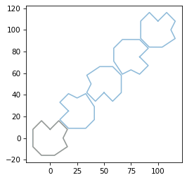
It should plot the asteroid at five locations between (0, 0) and (100, 100), and it should make about one full rotation.
plot_contour(a1.contour, color='C1')
for frame_num in range(0, 101, 25):
    transformed = transform_asteroid(a1, frame_num)
    plot_contour(transformed)
You can also use the following cells to animate the asteroid moving up and to the right.
def animate_asteroid(frame_num):
    transformed = transform_asteroid(a1, frame_num)
    asteroid_line.set_data(*transformed)
import matplotlib.animation as animation

fig, ax = plt.subplots()
#plt.plot([0, 100], [0, 100], '.')
[asteroid_line] = plt.plot([], [], alpha=0.5, color="C0")
ax.set_xlim(0, 100)
ax.set_ylim(0, 100)
ax.set_aspect('equal')

anim = animation.FuncAnimation(fig,
                               animate_asteroid,
                               frames=len(orbit),
                               interval=50)

plt.close(fig)
from IPython.display import HTML

HTML(anim.to_jshtml())
4.16.1. The Star Wars Crawl#
In the opening of Star Wars, text scrolls upward while shrinking toward a vanishing point. The effect is similar to a shear transform, but it is actually a projective transform, which is not an affine transform at all.
However, like affine transforms, it can be implemented using a 3x3 matrix and homogeneous coordinates, plus one extra step.
Here’s a function that makes the transform matrix, given a parameter, k.
def make_projection(k=0.1):
    return np.array([[1, 0, 0],
                     [0, 1, 0],
                     [0, k, 1]])
And here’s an example with a symbolic value of k.
k = symbols('k')
H = make_projection(k)
H
array([[1, 0, 0],
       [0, 1, 0],
       [0, k, 1]], dtype=object)
And here’s the effect on a vector in homogenous coordinates.
transformed = H @ v3
Matrix(transformed)
The result is no longer in valid homogeneous coordinates, but we can make it valid if divide through by w.
w = transformed[2]
scaled = transformed / w
Matrix(scaled)
The x and y coordinates are compressed by the factor \(k y + 1\), so points with larger y coordinates are compressed more.
The following function encapsulates these steps.
def projective_transform(contour, H):
    """Apply a 3x3 projective transform (homography) to a 2D contour.

    contour: (n,2) array of x,y coordinates
    H: 3x3 homography matrix

    Returns a transformed (n,2) array with perspective divide.
    """
    contour3 = augment_contour(contour)
    projected = H @ contour3.T
    return projected / projected[2]
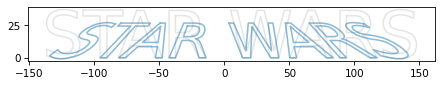
As an example, let’s create contours for the letters in “Star Wars” and apply a projective transform.
H = make_projection(0.01)
Here’s what the transformed text looks like, with the original text in the background.
contours = get_text_contours("STAR WARS", size=50)
for contour in contours:
    shifted = contour - [140, 0]
    plot_contour(shifted, color='gray', alpha=0.2)
    transformed = projective_transform(shifted, H)
    plot_contour(transformed)
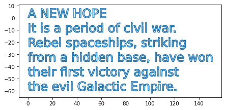
Here are the first few lines from the crawl of the first Star Wars movie.
text = """A NEW HOPE
It is a period of civil war.
Rebel spaceships, striking
from a hidden base, have won
their first victory against
the evil Galactic Empire."""
Here’s how we can get the contours for this text.
contours_list = [get_text_contours(line, size=10) for line in text.split('\n')]
And here’s what the results look like.
for i, contours in enumerate(contours_list):
    for contour in contours:
        shifted = contour - [0, 12 * i]
        xs, ys = shifted.T
        plt.plot(xs, ys, color='C0')
    decorate(aspect='equal')
Modify this code to apply a projective transform. As optional extensions, center the lines at zero so the transform is symmetric, and scale the lines horizontally so they are all the same width.
Copyright 2025 Allen B. Downey
Code license: MIT License
Text license: Creative Commons Attribution-NonCommercial-ShareAlike 4.0 International