DataFrames and Series

DataFrames and Series#

Click here to run this notebook on Colab.

from os.path import basename, exists

def download(url):
    filename = basename(url)
    if not exists(filename):
        from urllib.request import urlretrieve

        local, _ = urlretrieve(url, filename)
        print("Downloaded " + str(local))
    return filename

download('https://raw.githubusercontent.com/AllenDowney/ElementsOfDataScience/v1/utils.py')

import utils

This chapter introduces Pandas, a Python library that provides functions for reading and writing data files, exploring and analyzing data, and generating visualizations. And it provides two new types for working with data, DataFrame and Series.

We will use these tools to answer a data question – what is the average birth weight of babies in the United States? This example will demonstrate important steps in almost any data science project:

Identifying data that can answer a question.
Obtaining the data and loading it in Python.
Checking the data and dealing with errors.
Selecting relevant subsets from the data.
Using histograms to visualize a distribution of values.
Using summary statistics to describe the data in a way that best answers the question.
Considering possible sources of error and limitations in our conclusions.

Let’s start by getting the data.

Reading the Data#

To estimate average birth weight, we’ll use data from the National Survey of Family Growth (NSFG), which is available from the National Center for Health Statistics. To download the data, you have to agree to the Data User’s Agreement. URLs for the data and the agreement are in the notebook for this chapter.

The NSFG data is available from https://www.cdc.gov/nchs/nsfg.

The Data User’s Agreement is at https://www.cdc.gov/nchs/data_access/ftp_dua.htm.

You should read the terms carefully, but let me draw your attention to what I think is the most important one:

Make no attempt to learn the identity of any person or establishment included in these data.

NSFG respondents answer questions of the most personal nature with the expectation that their identities will not be revealed. As ethical data scientists, we should respect their privacy and adhere to the terms of use.

Respondents to the NSFG provide general information about themselves, which is stored in the respondent file, and information about each time they have been pregnant, which is stored in the pregnancy file.

We will work with the pregnancy file, which contains one row for each pregnancy and one column for each question on the NSFG questionnaire.

The data is stored in a fixed-width format, which means that every row is the same length and each column spans a fixed range of characters. For example, the first six characters in each row represent a a unique identifier for each respondent; the next two characters indicate whether a pregnancy is the respondent’s first, second, etc.

To read this data, we need a data dictionary, which specifies the names of the columns and the index where each one begins and ends. The data and the data dictionary are available in separate files. Instructions for downloading them are in the notebook for this chapter.

dict_file = '2015_2017_FemPregSetup.dct'
data_file = '2015_2017_FemPregData.dat'

Pandas can read data in most common formats, including CSV, Excel, and fixed-width format, but it cannot read the data dictionary, which is in Stata format. For that, we’ll use a Python library called statadict.

From statadict, we’ll import parse_stata_dict, which reads the data dictionary.

from statadict import parse_stata_dict

stata_dict = parse_stata_dict(dict_file)
stata_dict

<statadict.base.StataDict at 0x7fa5b87671f0>

The result is an object that contains

names, which is a list of column names, and
colspecs, which is a list of tuples, where each tuple contains the first and last index of a column.

These values are exactly the arguments we need to use read_fwf, which is the Pandas function that reads a file in fixed-width format.

import pandas as pd

nsfg = pd.read_fwf(data_file, 
                   names=stata_dict.names, 
                   colspecs=stata_dict.colspecs)
type(nsfg)

pandas.core.frame.DataFrame

The result from read_fwf() is a DataFrame, which is the primary type Pandas uses to store data. DataFrame has a method called head() that shows the first 5 rows:

nsfg.head()

	CASEID	PREGORDR	HOWPREG_N	HOWPREG_P	MOSCURRP	NOWPRGDK	PREGEND1	PREGEND2	HOWENDDK	NBRNALIV	...	SECU	SEST	CMINTVW	CMLSTYR	CMJAN3YR	CMJAN4YR	CMJAN5YR	QUARTER	PHASE	INTVWYEAR
0	70627	1	NaN	NaN	NaN	NaN	6.0	NaN	NaN	1.0	...	3	322	1394	1382	1357	1345	1333	18	1	2016
1	70627	2	NaN	NaN	NaN	NaN	1.0	NaN	NaN	NaN	...	3	322	1394	1382	1357	1345	1333	18	1	2016
2	70627	3	NaN	NaN	NaN	NaN	6.0	NaN	NaN	1.0	...	3	322	1394	1382	1357	1345	1333	18	1	2016
3	70628	1	NaN	NaN	NaN	NaN	6.0	NaN	NaN	1.0	...	2	366	1409	1397	1369	1357	1345	23	1	2017
4	70628	2	NaN	NaN	NaN	NaN	6.0	NaN	NaN	1.0	...	2	366	1409	1397	1369	1357	1345	23	1	2017

5 rows × 248 columns

The first two columns are CASEID and PREGORDR, which I mentioned earlier. The first three rows have the same CASEID, which means this respondent reported three pregnancies. The values of PREGORDR indicate that they are the first, second, and third pregnancies, in that order. We will learn more about the other columns as we go along.

In addition to methods like head, a Dataframe object has several attributes, which are variables associated with the object. For example, nsfg has an attribute called shape, which is a tuple containing the number of rows and columns:

nsfg.shape

(9553, 248)

There are 9553 rows in this dataset, one for each pregnancy, and 248 columns, one for each question. nsfg also has an attribute called columns, which contains the column names:

nsfg.columns

Index(['CASEID', 'PREGORDR', 'HOWPREG_N', 'HOWPREG_P', 'MOSCURRP', 'NOWPRGDK',
       'PREGEND1', 'PREGEND2', 'HOWENDDK', 'NBRNALIV',
       ...
       'SECU', 'SEST', 'CMINTVW', 'CMLSTYR', 'CMJAN3YR', 'CMJAN4YR',
       'CMJAN5YR', 'QUARTER', 'PHASE', 'INTVWYEAR'],
      dtype='object', length=248)

The column names are stored in an Index, which is another Pandas type, similar to a list.

Based on the names, you might be able to guess what some of the columns are, but in general you have to read the documentation. When you work with datasets like the NSFG, it is important to read the documentation carefully. If you interpret a column incorrectly, you can generate nonsense results and never realize it.

So, before we start looking at data, let’s get familiar with the NSFG codebook, which describes every column. You can download the codebook for this dataset from AllenDowney/ElementsOfDataScience.

If you search that document for “weigh at birth” you should find these columns related to birth weight.

BIRTHWGT_LB1: Birthweight in Pounds - 1st baby from this pregnancy
BIRTHWGT_OZ1: Birthweight in Ounces - 1st baby from this pregnancy

There are similar columns for a 2nd or 3rd baby, in the case of twins or triplets. For now we will focus on the first baby from each pregnancy, and we will come back to the issue of multiple births.

Series#

In many ways a DataFrame is like a Python dictionary, where the column names are the keys and the columns are the values. You can select a column from a DataFrame using the bracket operator, with a string as the key.

pounds = nsfg['BIRTHWGT_LB1']
type(pounds)

pandas.core.series.Series

The result is a Series, which is a Pandas type that represents a single column of data. In this case the Series contains the birth weight, in pounds, for each live birth.

head shows the first five values in the Series, the name of the Series, and the data type:

pounds.head()

  7.0
  NaN
  9.0
  6.0
  7.0
Name: BIRTHWGT_LB1, dtype: float64

One of the values is NaN, which stands for “Not a Number”. NaN is a special value used to indicate invalid or missing data. In this example, the pregnancy did not end in live birth, so birth weight is inapplicable.

Exercise: The column BIRTHWGT_OZ1 contains the ounces part of birth weight.

Select the column 'BIRTHWGT_OZ1' from nsfg and assign it to a new variable called ounces. Then display the first 5 elements of ounces.

Exercise: The Pandas types we have seen so far are DataFrame, Index, and Series. You can find the documentation of these types at:

This documentation can be overwhelming – I don’t recommend trying to read it all now. But you might want to skim it so you know where to look later.

Validation#

At this point we have identified the columns we need to answer the question and assigned them to variables named pounds and ounces.

pounds = nsfg['BIRTHWGT_LB1']
ounces = nsfg['BIRTHWGT_OZ1']

Before we do anything with this data, we have to validate it. One part of validation is confirming that we are interpreting the data correctly. We can use the value_counts method to see what values appear in pounds and how many times each value appears.

pounds.value_counts()

The values are in the left column and the counts are in the right column. By default, the results are sorted with the highest count first, but we can use sort_index to sort them by value instead, with the lightest babies first and heaviest babies last.

pounds.value_counts().sort_index()

BIRTHWGT_LB1
0        2
0       28
0       46
0       76
0      179
0      570
0     1644
0     2268
0     1287
0      396
0      82
0      17
0       2
0       1
0       1
0       2
0      89
Name: count, dtype: int64

As we’d expect, the most frequent values are 6-8 pounds, but there are some very light babies, a few very heavy babies, and two special values, 98, and 99. According to the codebook, these values indicate that the respondent declined to answer the question (98) or did not know (99).

We can validate the results by comparing them to the codebook, which lists the values and their frequencies.

value	label	Total
.	INAPPLICABLE	2863
0-5	UNDER 6 POUNDS	901
6	6 POUNDS	1644
7	7 POUNDS	2268
8	8 POUNDS	1287
9-95	9 POUNDS OR MORE	499
98	Refused	2
99	Don’t know	89
	Total	9553

The results from value_counts agree with the codebook, so we have some confidence that we are reading and interpreting the data correctly.

Exercise: In nsfg, the column 'OUTCOME' encodes the outcome of each pregnancy as shown below:

Value	Meaning
1	Live birth
2	Induced abortion
3	Stillbirth
4	Miscarriage
5	Ectopic pregnancy
6	Current pregnancy

Use value_counts to display the values in this column and how many times each value appears. Are the results consistent with the codebook?

Summary Statistics#

Another way to validate the data is with describe, which computes statistics that summarize the data, like the mean, standard deviation, minimum, and maximum. Here are the results for pounds.

pounds.describe()

count    6690.000000
mean        8.008819
std        10.771360
min         0.000000
25%         6.000000
50%         7.000000
75%         8.000000
max        99.000000
Name: BIRTHWGT_LB1, dtype: float64

count is the number of values, not including NaN. In this column, there are 6690 value that are not NaN. mean and std are the mean and standard deviation. min and max are the minimum and maximum values, and in between are the 25th, 50th, and 75th percentiles. The 50th percentile is the median.

The mean is about 8.05, but that doesn’t mean much because it includes the special values 98 and 99. Before we can really compute the mean, we have to replace those values with NaN to identify them as missing data. The replace() method does what we want:

import numpy as np

pounds_clean = pounds.replace([98, 99], np.nan)

replace takes a list of the values we want to replace and the value we want to replace them with. np.nan means we are getting the special value NaN from the NumPy library, which is imported as np. The result from replace() is a new Series, which I assign to pounds_clean. If we run describe again, we see that count is smaller now because it includes only the valid values.

pounds_clean.describe()

count    6599.000000
mean        6.754357
std         1.383268
min         0.000000
25%         6.000000
50%         7.000000
75%         8.000000
max        14.000000
Name: BIRTHWGT_LB1, dtype: float64

The mean of the new Series is about 6.7 pounds. Remember that the mean of the original Series was more than 8 pounds. It makes a big difference when you remove a few 99-pound babies!

Exercise: Use describe to summarize ounces.
Then use replace to replace the special values 98 and 99 with NaN, and assign the result to ounces_clean. Run describe again. How much does this cleaning affect the results?

Series Arithmetic#

Now we want to combine pounds and ounces into a single Series that contains total birth weight. Arithmetic operators work with Series objects – for example, to convert pounds to ounces, we could write

pounds * 16

Then we could add in ounces like this

pounds * 16 + ounces

Exercise: Use pounds_clean and ounces_clean to compute the total birth weight expressed in kilograms (there are roughly 2.2 pounds per kilogram). What is the mean birth weight in kilograms?

Histograms#

Let’s get back to the original question: what is the average birth weight for babies in the U.S.?
As an answer we could take the results from the previous section and compute the mean:

pounds_clean = pounds.replace([98, 99], np.nan)
ounces_clean = ounces.replace([98, 99], np.nan)

birth_weight = pounds_clean + ounces_clean / 16
birth_weight.mean()

7.180217889908257

But it is risky to compute a summary statistic, like the mean, before we look at the whole distribution of values. A distribution is a set of possible values and their frequencies. One way to visualize a distribution is a histogram, which shows values on the x axis and their frequencies on the y axis. Series provides a hist method that makes histograms, and we can use Pyplot to label the axes.

import matplotlib.pyplot as plt

birth_weight.hist(bins=30)
plt.xlabel('Birth weight in pounds')
plt.ylabel('Number of live births')
plt.title('Distribution of U.S. birth weight');

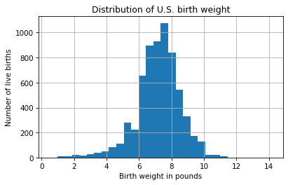
_images/457a86aaf2898cf0286465175b6f73f97f3f3b1feab017475be1b114109f9e51.png

The keyword argument, bins, tells hist to divide the range of weights into 30 intervals, called bins, and count how many values fall in each bin. The x axis is birth weight in pounds; the y axis is the number of births in each bin.

The distribution looks like a bell curve, but the tail is longer on the left than on the right – that is, there are more light babies than heavy babies. That makes sense, because the distribution includes some babies that were born preterm.

Exercise: hist takes keyword arguments that specify the type and appearance of the histogram. Find the documentation of hist and see if you can figure out how to plot the histogram as an unfilled line against a background with no grid lines.

Exercise: The NSFG dataset includes a column called AGECON that records a woman’s age at conception for each pregnancy.

Select this column from the DataFrame and plot the histogram of the values with 20 bins.
Label the x and y axes appropriately.

Boolean Series#

We have seen that the distribution of birth weights is skewed to the left – that is, there are more light babies than heavy ones and they are farther from the mean. That’s because preterm babies tend to be lighter. The most common duration for pregnancy is 39 weeks, which is “full term”; “preterm” is usually defined to be less than 37 weeks.

To see which babies are preterm, we can use the PRGLNGTH column, which records pregnancy length in weeks.

preterm = (nsfg['PRGLNGTH'] < 37)
preterm.dtype

dtype('bool')

When you compare a Series to a value, the result is a Boolean Series – that is, a Series where each element is a Boolean value, True or False. In this case, it’s True for each preterm baby and False otherwise. We can use head to see the first 5 elements.

preterm.head()

  False
   True
  False
  False
  False
Name: PRGLNGTH, dtype: bool

If you compute the sum of a Boolean Series, it treats True as 1 and False as 0, so the sum is the number of True values, which is the number of preterm babies.

preterm.sum()

If you compute the mean of a Boolean Series, you get the fraction of True values. In this case, it’s about 0.38 – that is, about 38% of the pregnancies are less than 37 weeks.

preterm.mean()

0.38469590704490736

However, this result might be misleading because it includes all pregnancy outcomes, not just live births. We can create another Boolean Series to indicate which pregnancies ended in live birth:

live = (nsfg['OUTCOME'] == 1)
live.mean()

0.7006176070344394

Now we can use the operator &, which represents the logical AND operation, to identify pregnancies where the outcome is a live birth and preterm:

live_preterm = (live & preterm)
live_preterm.mean()

0.08929132209777034

About \(9\%\) of all pregnancies resulted in a preterm live birth.

The other common logical operators that work with Series objects are:

|, which represents the logical OR operation – for example, live | preterm is true if either live is true, or preterm is true, or both.
~, which represents the logical NOT operation – for example, ~live is true if live is false or NaN.

The logical operators treat NaN the same as False, so you should be careful about using the NOT operator with a Series that contains NaN values. For example, ~preterm would include not just full term pregnancies, but also pregnancies with unknown length.

Exercise: Of all pregnancies, what fraction are live births at full term (37 weeks or more)? Of all live births, what fraction are full term?

Filtering Data#

We can use a Boolean Series as a filter – that is, we can select only rows that satisfy a condition or meet some criterion. For example, we can use preterm and the bracket operator to select values from birth_weight, so preterm_weight gets birth weights for preterm babies.

preterm_weight = birth_weight[preterm]
preterm_weight.mean()

5.480958781362007

To select full-term babies, we can create a Boolean Series like this:

fullterm = (nsfg['PRGLNGTH'] >= 37)

And use it to select birth weights for full term babies:

full_term_weight = birth_weight[fullterm]
full_term_weight.mean()

7.429609416096791

As expected, full term babies are heavier, on average, than preterm babies. To be more explicit, we could also limit the results to live births, like this:

full_term_weight = birth_weight[live & fullterm]
full_term_weight.mean()

7.429609416096791

But in this case we get the same result because birth_weight is only valid for live births.

Exercise: Let’s see if there is a difference in weight between single births and multiple births (twins, triplets, etc.). The column NBRNALIV represents the number of babies born alive from a single pregnancy.

nbrnaliv = nsfg['NBRNALIV']
nbrnaliv.value_counts()

NBRNALIV
1.0    6573
2.0     111
3.0       6
Name: count, dtype: int64

Use nbrnaliv and live to create a Boolean series called multiple that is true for multiple live births. Of all live births, what fraction are multiple births?

Exercise: Make a Boolean series called single that is true for single live births. Of all single births, what fraction are preterm? Of all multiple births, what fraction are preterm?

Exercise: What is the average birth weight for live, single, full-term births?

Weighted Means#

We are almost done, but there’s one more problem we have to solve: oversampling.

The NSFG sample is not exactly representative of the U.S. population. By design, some groups are more likely to appear in the sample than others – that is, they are oversampled. Oversampling helps to ensure that you have enough people in every group to get reliable statistics, but it makes data analysis a little more complicated.

Each pregnancy in the dataset has a sampling weight that indicates how many pregnancies it represents. In nsfg, the sampling weight is stored in a column named wgt2015_2017. Here’s what it looks like.

sampling_weight = nsfg['WGT2015_2017']
sampling_weight.describe()

count      9553.000000
mean      13337.425944
std       16138.878271
min        1924.916000
25%        4575.221221
50%        7292.490835
75%       15724.902673
max      106774.400000
Name: WGT2015_2017, dtype: float64

The median value (50th percentile) in this column is about 7292, which means that a pregnancy with that weight represents 7292 total pregnancies in the population. But the range of values is wide, so some rows represent many more pregnancies than others.

To take these weights into account, we can compute a weighted mean. Here are the steps:

Multiply the birth weights for each pregnancy by the sampling weights and add up the products.
Add up the sampling weights.
Divide the first sum by the second.

To do this correctly, we have to be careful with missing data. To help with that, we’ll use two Series methods, isna and notna. isna returns a Boolean Series that is True where the corresponding value is NaN.

missing = birth_weight.isna()
missing.sum()

In birth_weight there are 3013 missing values (mostly for pregnancies that did not end in live birth). notna returns a Boolean Series that is True where the corresponding value is not NaN.

valid = birth_weight.notna()
valid.sum()

We can combine valid with the other Boolean Series we have computed to identify single, full term, live births with valid birth weights.

single = (nbrnaliv == 1)
selected = valid & live & single & fullterm
selected.sum()

You can finish off this computation as an exercise.

Exercise: Use selected, birth_weight, and sampling_weight to compute the weighted mean of birth weight for live, single, full term births. You should find that the weighted mean is a little higher than the unweighted mean we computed in the previous section. That’s because the groups that are oversampled in the NSFG tend to have lighter babies, on average.

Making an Extract#

The NSFG dataset is large, and reading a fixed-width file is relatively slow. So now that we’ve read it, let’s save a smaller version in a more efficient format. When we come back to this dataset in Chapter 13, here are the columns we’ll need.

variables = ['CASEID', 'OUTCOME', 'BIRTHWGT_LB1', 'BIRTHWGT_OZ1',
             'PRGLNGTH', 'NBRNALIV', 'AGECON', 'AGEPREG', 'BIRTHORD',
             'HPAGELB', 'WGT2015_2017']

And here’s how we can select just those columns from the DataFrame.

subset = nsfg[variables]
subset.shape

(9553, 11)

DataFrame provides several methods for writing data to a file – the one we’ll use is to_hdf, which creates an HDF file. The parameters are the name of the new file, the name of the object we’re storing in the file, and the compression level, which determines how effectively the data are compressed.

filename = 'nsfg.hdf'
nsfg.to_hdf(filename, 'nsfg', complevel=6)

The result is much smaller than the original fixed-width file, and faster to read. We can read it back like this.

nsfg = pd.read_hdf(filename, 'nsfg')

Summary#

This chapter poses what seems like a simple question: what is the average birth weight of babies in the United States?

To answer it, we found an appropriate dataset and downloaded the files. We used Pandas to read the files and create a DataFrame. Then we validated the data and dealt with special values and missing data. To explore the data, we used value_counts, hist, describe, and other methods. And to select relevant data, we used Boolean Series objects.

Along the way, we had to think more about the question. What do we mean by “average”, and which babies should we include? Should we include all live births or exclude preterm babies or multiple births?

And we had to think about the sampling process. By design, the NSFG respondents are not representative of the U.S. population, but we can use sampling weights to correct for this effect.

Even a simple question can be a challenging data science project.

A note on vocabulary: In a dataset like the one we used in this chapter, we could say that each column represents a “variable”, and what we called column names might also be called variable names. I avoided that use of the term because it might be confusing to say that we select a “variable” from a DataFrame and assign it to a Python variable. But you might see this use of the term elsewhere, so I thought I would mention it.