Testing percentiles#
Here’s a question from the Reddit statistics forum.
I have two different samples (about 100 observations per sample) drawn from the same population (or that’s what I hypothesize; the populations may in fact be different). The samples and population are approximately normal in distribution.
I want to estimate the 85th percentile value for both samples, and then see if there is a statistically significant difference between these two values. I cannot use a normal z- or t-test for this, can I? It’s my current understanding that those tests would only work if I were comparing the means of the samples.
As an extension of this, say I wanted to compare one of these 85th percentile values to a fixed value; again, if I was looking at the mean, I would just construct a confidence interval and see if the fixed value fell within it…but the percentile stuff is throwing me for a loop.
This is […] related to a research project I’m working on (in my job).
There are two questions here. The first is about testing a difference in percentiles between two groups. The second is about the difference between a percentile from an observed sample and an expected value.
We’ll answer the first question with a permutation test, and we’ll answer the second in two ways: bootstrap resampling and a Gaussian model.
Click here to run this notebook on Colab.
I’ll download a utilities module with some of my frequently-used functions, and then import the usual libraries.
from os.path import basename, exists

def download(url):
    filename = basename(url)
    if not exists(filename):
        from urllib.request import urlretrieve

        local, _ = urlretrieve(url, filename)
        print("Downloaded " + str(local))
    return filename

download('https://github.com/AllenDowney/DataQnA/raw/main/nb/utils.py')

import numpy as np
import matplotlib.pyplot as plt
import pandas as pd
import seaborn as sns

from utils import decorate
Show code cell content
# install the empiricaldist library, if necessary

try:
    import empiricaldist
except ImportError:
    !pip install empiricaldist
Data#
Since OP didn’t provide a dataset, we have to generate one. I’ll draw two samples from Gaussian distributions with the same standard deviation and different means.
np.random.seed(17)

mu = 10
sigma = 2
size = 100

group1 = np.random.normal(mu, sigma, size=size)
group2 = np.random.normal(mu+1, sigma, size=size)
Here’s what the distributions of the groups look like.
sns.kdeplot(group1, label='Group1')
sns.kdeplot(group2, label='Group2')

decorate(xlabel='Quantity',
         ylabel='Density',
         title='Distributions of the data')
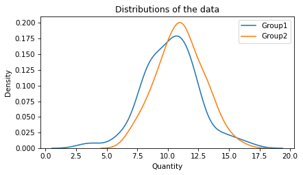
If we compute the 85th percentile in both groups, we see a difference, as expected.
stat1 = np.percentile(group1, 85)
actual_stat2 = np.percentile(group2, 85)
stat1, actual_stat2
(12.241826987876475, 13.057003640622057)
actual_diff = actual_stat2 - stat1
actual_diff
0.8151766527455813
Now let’s see if a difference of that size would be likely if the two samples were actually drawn from the same distribution.
Testing the Difference#
When we test a difference between two groups, the usual model of the null hypothesis is that the groups are actually identical. If that’s true, the two samples came from the same distribution, so we can combine them into a single sample.
pooled = np.concatenate([group1, group2])
n, m = len(group1), len(group2)
Now we can simulate the null hypothesis by permutation – that is, by shuffling the pooled data and splitting it into two groups with the same sizes as the originals. The following function generates two samples under this assumption, and returns the difference in their 85th percentiles.
def simulate_percentile_difference():
    np.random.shuffle(pooled)
    shuffled1 = pooled[:n]
    shuffled2 = pooled[n:]
    diff = np.percentile(shuffled1, 85) - np.percentile(shuffled2, 85)
    return diff
If we call it many times, the result is a sample from the distribution of differences under the null hypothesis.
np.random.seed(19)
sample_diff = [simulate_percentile_difference() for i in range(1001)]
Here’s what it looks like, with a vertical line at the observed difference.
I’m plotting it with cut=0 so the estimated density doesn’t extend past the minimum and maximum of the data.
sns.kdeplot(sample_diff, label='', cut=0)
plt.axvline(actual_diff, ls=':', color='gray')
decorate(xlabel='Difference',
         ylabel='Density',
         title='Distribution of differences under H0')
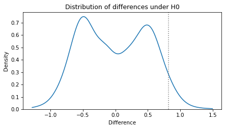
The distribution is multimodal, which is the result of selecting a moderately high percentile from a moderately small dataset – the diversity of the results is limited. However, in this example we are interested in the tails of the distribution, so multimodality is not a problem.
To estimate a one-sided p-value, we can compute the fraction of the sample that exceeds the actual difference.
p_value_one_sided = (sample_diff >= actual_diff).mean()
p_value_one_sided
0.04195804195804196
Or, for a two-sided p-value, we can compute the fraction of the sample that exceeds the actual difference in absolute value.
p_value_two_sided = (np.abs(sample_diff) > actual_diff).mean()
p_value_two_sided
0.07892107892107893
In this example, the result of the one-sided test would be considered significant at the 5% significance level, but the two-sided test would not. So which is it?
I think it’s not worth worrying about. My interpretation of the results is the same either way: they are inconclusive. Under the null hypothesis, a difference as big as the one we saw would be unlikely, but we can’t rule out the possibility that the groups are identical – or nearly so – and the apparent difference is due to random variation.
Testing a fixed value#
Now let’s turn to the second question. Suppose we have reason to think that the actual value of the 85th percentile is 12.3, and we would like to know whether the data contradict this hypothesis.
expected = 12.3
We’ll test group1 first.
Here’s the 85th percentile of group1 and its difference from the expected value.
actual_stat1 = np.percentile(group1, 85)
actual_diff1 = actual_stat1 - expected
actual_stat1, actual_diff1
(12.241826987876475, -0.058173012123525325)
Let’s see if a difference of this magnitude is likely to happen under the null hypothesis. One way to model the null hypothesis is to create a dataset that is similar to the observed data, but where the 85th percentile is exactly as expected. We can do that by shifting the observed data by the observed difference.
shifted = group1 - actual_diff1
np.percentile(shifted, 85)
12.3
The 85th percentile of the shifted data is the expected value, exactly.
Now, to generate samples under the null hypothesis, we can use the following function, which takes a sample, shifts it to have the expected value of the 85th percentile, generates a bootstrap resample of the shifted values, and returns the difference between the 85th percentile of the sample and the expected value.
def bootstrap_percentile(group):
    stat = np.percentile(group, 85) - expected
    shifted = group - stat
    resampled = np.random.choice(shifted, size=len(group), replace=True)
    return np.percentile(resampled, 85) - expected
If we call this function many times, we get a sample of the differences we expect under the null hypothesis.
np.random.seed(17)
sample1 = [bootstrap_percentile(group1) for i in range(1001)]
The following function shows the distribution of the sample with a vertical line at the observed value.
sns.kdeplot(sample1, label='Sampling distribution')
plt.axvline(actual_diff1, ls=':', color='gray')
decorate(xlabel='Deviation',
         ylabel='Density',
         title='Distribution of deviations from expected under H0')
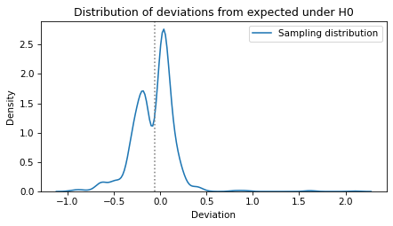
Without computing a p-value, we can see that a difference as big as actual_diff1 is entirely plausible under the null hypothesis.
We can confirm that by computing a one-sided p-value.
p_value_one_side = (sample1 < actual_diff1).mean()
p_value_one_side
0.4405594405594406
So the observed difference in the first group is not statistically significant. Now let’s do the same thing for the second group.
actual_stat2 = np.percentile(group2, 85)
actual_diff2 = actual_stat2 - expected
actual_diff2
0.7570036406220559
np.random.seed(17)
sample2 = [bootstrap_percentile(group2) for i in range(1001)]
Here’s what the distribution of differences looks like under the null hypothesis, with a vertical line at the observed value.
sns.kdeplot(sample2, label='Group 2', cut=0)
plt.axvline(actual_diff2, ls=':', color='gray')
decorate(xlabel='Deviation',
         ylabel='Density',
         title='Distribution of deviations from expected under H0')
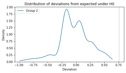
There are no differences in the sample that exceed the observed value.
np.max(sample2), actual_diff2
(0.6391539586773582, 0.7570036406220559)
We can conclude that a difference as big as that is very unlikely under the null hypothesis. There’s not much point in computing a p-value more precisely than that, but if it’s required, we can estimate it if we assume that the tail of the sampling distribution is roughly Gaussian. In that case, we can fit a KDE to the sampling distribution like this.
from scipy.stats import gaussian_kde

kde = gaussian_kde(sample2)
And use a Pmf object to approximate the estimated density.
from empiricaldist import Pmf

qs = np.linspace(-2, 2, 201)
ps = kde.evaluate(qs)
pmf = Pmf(ps, qs)
pmf.normalize()
49.99999999999998
Then we can use the corresponding CDF to compute the probability of a value that exceeds the observed difference.
cdf = pmf.make_cdf()
p_value = 1 - cdf(actual_diff)
p_value
3.319666203671634e-05
So the p-value is quite small.
Model-based resampling#
The bootstrap method in the previous section is a good choice if we are unsure about the distribution of the data, or if there are outliers. But multiple modes in the sampling distribution suggest that there might not be enough diversity in the data for bootstrapping to be reliable.
Fortunately, there is another way we might model the null hypothesis: using a Gaussian distribution. If we generate data from a continuous distribution, we expect the sampling distribution to be unimodal.
But there is a problem we have to solve first – we have to make an assumption about the standard deviation of the hypothetical Gaussian distribution. One option is to use the standard deviation of the data.
s = np.std(group1)
Now we need to find a Gaussian distribution with a given standard deviation that has the expected 85th percentile. We can do that by starting with a distribution centered at 0, computing it’s 85th percentile and then shifting it.
from scipy.stats import norm

dist0 = norm(0, s)
quantity = dist0.ppf(0.85)
quantity
2.3232308032911324
ppf stands for “percentile point function”, which is another name for the quantile function, which is the inverse of the CDF – it takes a cumulative probability and returns the corresponding quantity.
center = expected - quantity
dist = norm(center, s)
dist.ppf(0.85)
12.3
The following function takes one of the groups, fits a hypothetical model to it, generates a sample from the model, and returns the difference between the 85th percentile of the sample and the expected value.
def gaussian_percentile(group):
    s = np.std(group)
    dist0 = norm(0, s)
    quantity = dist0.ppf(0.85)
    center = expected - quantity
    dist = norm(center, s)
    sample = dist.rvs(size=len(group))
    return np.percentile(sample, 85) - expected
If we call this function many times, we get the sampling distribution of the test statistic under the null hypothesis.
np.random.seed(17)
sample3 = [gaussian_percentile(group1) for i in range(1001)]
Here’s what the distribution looks like, compared to the corresponding distribution from the bootstrapped model.
sns.kdeplot(sample1, label='Bootstrap model', cut=0)
sns.kdeplot(sample3, label='Gaussian model', cut=0)
plt.axvline(actual_diff1, ls=':', color='gray')
decorate(xlabel='Quantity',
         ylabel='Density',
         title='Distribution of deviations from expected under H0, Group 1')
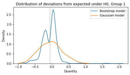
The shapes of the distributions are different, but their ranges are comparable.
And the conclusion is the same: a difference as big as actual_diff1 is entirely plausible under the null hypothesis.
p_value_one_side = (sample3 < actual_diff1).mean()
p_value_one_side
0.48451548451548454
Now let’s try the same test with Group 2.
np.random.seed(17)
sample4 = [gaussian_percentile(group2) for i in range(1001)]
Here’s the result, along with the result from the bootstrap model.
sns.kdeplot(sample2, label='Bootstrap model', cut=0)
sns.kdeplot(sample4, label='Gaussian model', cut=0)
plt.axvline(actual_diff2, ls=':', color='gray')
decorate(xlabel='Quantity',
         ylabel='Density',
         title='Distribution of deviations from expected under H0, Group 2')
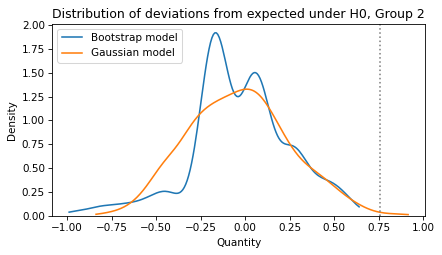
Again, the shapes of the distributions are different, but the conclusion is the same.
A difference as big as actual_diff2 is unlikely under the null hypothesis.
p_value_one_side = (sample4 > actual_diff2).mean()
p_value_one_side
0.003996003996003996
As usual, the two-sided p-value is bigger by a factor of two, roughly, but the difference never matters in practice.
p_value_two_sided = (np.abs(sample4) > actual_diff2).mean()
p_value_two_sided
0.006993006993006993
Under this model of the null hypothesis, the probability is small that the 85th percentile of the data would exceed the expected value by so much.
Discussion#
This example demonstrates a kind of inconsistency in hypothesis testing. We found that Group 1 is not significantly different from the expected value – in the technical sense of significantly – but Group 2 is. So that suggests that Group 1 and Group 2 are different from each other, but when we test that hypothesis, the difference is not statistically significant.
People who are new to hypothesis testing find results like this surprising, but they are not rare. Generally, they are a consequence of the logic of null hypothesis testing and the arbitrariness of the significance threshold.
I think it helps to interpret p-values qualitatively.
A p-value greater than 10% means that the observed effect is plausible under the null hypothesis, and could happen by chance.
A p-value less than 1% means that an observed effect is unlikely under the null hypothesis – so it is unlikely to have happened by chance.
Anything in between is inconclusive.
There is nothing special about 5%.
Data Q&A: Answering the real questions with Python
Copyright 2024 Allen B. Downey
License: Creative Commons Attribution-NonCommercial-ShareAlike 4.0 International