Sample Size Selection

Here’s a question from the Reddit statistics forum.

Hi Redditors, I am a civil engineer trying to solve a statistical problem for a current project I have. I have a pavement parking lot 125,000 sf in size. I performed nondestructive testing to render an opinion about the areas experiencing internal delimitation not observable from the surface. Based on preliminary testing, it was determined that 9% of the area is bad, and 11% of the total area I am unsure about (nonconclusive results if bad or good), and 80% of the area is good. I need to verify all areas using destructive testing, I will take out slabs 2 sf in size. my question is how many samples do I need to take from each area to confirm the results with 95% confidence interval?

There are elements of this question that are not clear, and OP did not respond to follow-up questions. But the question is generally about sample size selection, so let’s talk about that.

If the parking lot is 125,000 sf and each sample is 2 sf, we can imagine dividing the total area into 62,500 test patches. Of those, some unknown proportion are good and the rest are bad.

In reality, there is probably some spatial correlation – if a patch is bad, the nearby patches are more likely to be bad. But if we choose a sample of patches entirely at random, we can assume that they are independent. In that case, we can estimate the proportion of patches that are good and quantify the precision of that estimate by computing a confidence interval.

Then we can choose a sample size that meets some requirement. For example, we might want the 95% confidence interval to be smaller than a given threshold, or we might want to bound the probability that the proportion falls below some threshold.

But let’s start by estimating proportions and computing confidence intervals.

Click here to run this notebook on Colab.

I’ll download a utilities module with some of my frequently-used functions, and then import the usual libraries.

from os.path import basename, exists

def download(url):
    filename = basename(url)
    if not exists(filename):
        from urllib.request import urlretrieve

        local, _ = urlretrieve(url, filename)
        print("Downloaded " + str(local))
    return filename

download('https://github.com/AllenDowney/DataQnA/raw/main/nb/utils.py')

import numpy as np
import matplotlib.pyplot as plt
import pandas as pd
import seaborn as sns

from utils import decorate

Show code cell content Hide code cell content

# install the empiricaldist library, if necessary

try:
    import empiricaldist
except ImportError:
    !pip install empiricaldist

The beta-binomial model

Based on preliminary testing, it is likely that the proportion of good patches is between 80% and 90%. We can take advantage of that information by using a beta distribution as a prior and updating it with the data. Here’s a prior distribution that seems like a reasonable choice, given the background information.

from scipy.stats import beta as beta_dist

prior = beta_dist(8, 2)
prior.mean()

0.8

The prior mean is at the low end of the likely range, so the results will be a little conservative. Here’s what the prior looks like.

def plot_dist(dist, **options):
    qs = np.linspace(0, 1, 101)
    ps = dist.pdf(qs)
    ps /= ps.sum()
    plt.plot(qs, ps, **options)

plot_dist(prior, color='gray', label='prior')

decorate(xlabel='Proportion good',
         ylabel='PDF')

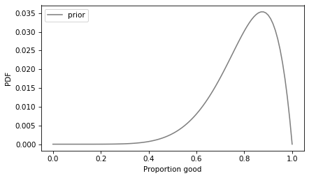
This prior leaves open the possibility of values below 80% and greater than 90%, but it assigns them lower probabilities.

Now let’s generate a hypothetical dataset to see what the update looks like. Suppose the actual percentage of good patches is 90%, and we sample n=10 of them.

def generate_data(n, p):
    yes = int(round(n * p))
    no = n - yes
    return yes, no

And suppose that, in line with expectations, 9 out of 10 tests are good.

yes, no = generate_data(n=10, p=0.9)
yes, no

(9, 1)

Under the beta-binomial model, computing the posterior is easy.

def update(dist, yes, no):
    a, b = dist.args
    return beta_dist(a + yes, b + no)

Here’s how we run the update.

posterior10 = update(prior, yes, no)
posterior10.mean()

0.85

The posterior mean is 85%, which is half way between the prior mean and the proportion observed in the data.

Here’s what the posterior distribution looks like, compared to the prior.

plot_dist(prior, color='gray', label='prior')
plot_dist(posterior10, label='posterior10')

decorate(xlabel='Proportion good',
         ylabel='PDF')

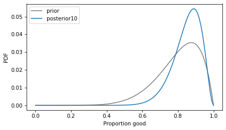
Given the posterior distribution, we can use ppf, which computes the inverse CDF, to compute a confidence interval.

def confidence_interval(dist, percent=95):
    low = (100 - percent) / 200
    high = 1 - low
    ci = dist.ppf([low, high])
    return ci

Here’s the result for this example.

confidence_interval(posterior10)

array([0.66862334, 0.96617375])

With a sample size of only 10, the confidence interval is still quite wide – that is, the estimate of the proportion is not precise.

More data?

Now let’s run the same analysis with a sample size of n=100.

yes, no = generate_data(n=100, p=0.9)
posterior100 = update(prior, yes, no)
posterior100.mean()

0.8909090909090909

With a larger sample size, the posterior mean is closer to the proportion observed in the data. And the posterior distribution is narrower, which indicates greater precision.

plot_dist(prior, color='gray', label='prior')
plot_dist(posterior10, label='posterior10')
plot_dist(posterior100, label='posterior100')

decorate(xlabel='Proportion good',
         ylabel='PDF')

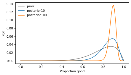
The confidence interval is much smaller.

confidence_interval(posterior100)

array([0.82660267, 0.94180387])

If we need more precision than that, we can increase the sample size more. If we don’t need that much precision, we can decrease it.

With some math, we could compute the sample size algorithmically, but a simple alternative is to run this analysis with different sample sizes until we get the results we need.

But what about that prior?

Some people don’t like using Bayesian methods because they think it is more objective to ignore perfectly good background information, even in cases like this where they come from preliminary testing that is clearly applicable.

To satisfy them, we can run the analysis again with a uniform prior, which is not actually more objective, but it seems to make people happy.

uniform_prior = beta_dist(1, 1)
uniform_prior.mean()

0.5

The mean of the uniform prior is 50%, so it is more pessimistic. Here’s the update with n=10.

yes, no = generate_data(n=10, p=0.9)
uniform_posterior10 = update(uniform_prior, yes, no)
uniform_posterior10.mean()

0.8333333333333334

Now let’s compare the posterior distributions with the informative prior and the uniform prior.

plot_dist(uniform_prior, color='gray', label='uniform prior')
plot_dist(posterior10, color='C1', label='posterior10')
plot_dist(uniform_posterior10, color='C4', label='uniform posterior10')

decorate(xlabel='Proportion good',
         ylabel='PDF')

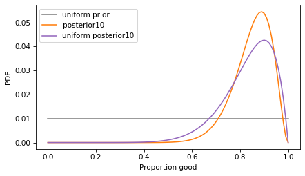
With the informative prior, the posterior distribution is a little narrower – an estimate that uses background information is more precise.

Let’s do the same thing with n=100.

uniform_prior = beta_dist(1, 1)
yes, no = generate_data(n=100, p=0.9)
uniform_posterior100 = update(uniform_prior, yes, no)

plot_dist(uniform_prior, color='gray', label='uniform prior')
plot_dist(posterior100, color='C1', label='posterior100')
plot_dist(uniform_posterior100, color='C4', label='uniform posterior100')

decorate(xlabel='Proportion good',
         ylabel='PDF')

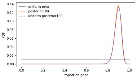
With a larger sample size, the choice of the prior has less effect – the posterior distributions are almost the same.

Discussion

Sample size analysis is a good thing to do when you are designing experiments, because it requires you to

• Make a model of the data-generating process,

• Generate hypothetical data, and

• Specify ahead of time what analysis you plan to do.

It also gives you a preview of what the results might look like, so you can think about the requirements. If you do these things before running an experiment, you are likely to clarify your thinking, communicate better, and improve the data collection process and analysis.

Sample size analysis can also help you choose a sample size, but most of the time that’s determined by practical considerations, anyway. I mean, how many holes do you think they’ll let you put in that parking lot?

Data Q&A: Answering the real questions with Python

Copyright 2024 Allen B. Downey

License: Creative Commons Attribution-NonCommercial-ShareAlike 4.0 International