Estimation with Small Samples

Here’s a question from the Reddit statistics forum.

Hey, so imagine I only have 6 samples from a value that has a normal distribution. Can I estimate the range of likely distributions from those 6?

Let’s be more specific. I’m considering the accuracy of a blood testing device. I took 6 samples of my blood at the same time from the same vein and gave them to the machine. The results are not all the same (as expected), indicating the device’s inherent level of imprecision.

So, I’m wondering if there’s a way to estimate the range of possibilities of what I would see if I could give 100 or 1000 samples?

I’m comfortable assuming a normal distribution around the “true” value. Is there any stats method to guesstimate the range of likely values for sigma? Or would I just need to drain my blood dry to get 1000 samples to figure that out?

Fyi, not a statistician.

Because the sample size is so small, this question cries out for a Bayesian approach. Why?

• Bayesian methods do a good job of taking advantage of background information and extracting as much information as possible from the data,

• With a small sample size, the uncertainty of the result is large, so it is important to quantify it, and

• The motivating question is explicitly about making probabilistic predictions, which is what Bayesian methods do and classical methods don’t.

As an example, OP suggested looking at blood potassium (K+) levels, with the following data:

4.0, 3.9, 4.0, 4.0, 4.7, 4.2 (mmol/L)

OP also explained that the blood samples were collected “continuously from a single puncture … within seconds, not minutes,” so we don’t expect the true level to change much between samples. In that case, the variation in the measurements would largely reflect the precision of the testing device.

With that assumption, let’s see what we can do.

Click here to run this notebook on Colab.

I’ll download a utilities module with some of my frequently-used functions, and then import the usual libraries.

Show code cell content Hide code cell content

from os.path import basename, exists

def download(url):
    filename = basename(url)
    if not exists(filename):
        from urllib.request import urlretrieve

        local, _ = urlretrieve(url, filename)
        print("Downloaded " + str(local))
    return filename

download('https://github.com/AllenDowney/DataQnA/raw/main/nb/utils.py')

import numpy as np
import matplotlib.pyplot as plt
import pandas as pd
import seaborn as sns

from utils import decorate

Show code cell content Hide code cell content

# install the empiricaldist library, if necessary

try:
    import empiricaldist
except ImportError:
    !pip install empiricaldist

Bayesian estimation

Here’s the data.

data = [4.0, 3.9, 4.0, 4.0, 4.7, 4.2]
np.mean(data), np.std(data)

(4.133333333333334, 0.2687419249432851)

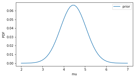
Now we need prior distributions for mu and sigma. For the prior distribution of mu we can use the distribution in the general population. The “normal range” for potassium – which is usually the 5th and 95th percentiles of the population – is 3.5 to 5.4 mmol/L. So we can construct a normal distribution with these percentiles.

from scipy.stats import norm

hyper_mu = (3.5 + 5.4) / 2
hyper_sigma = 0.6

dist = norm(hyper_mu, hyper_sigma)
dist.ppf([0.05, 0.95])

array([3.46308782, 5.43691218])

Now I’ll make a Pmf object that represents this distribution.

mus = np.linspace(2, 7, 51)
ps = dist.pdf(mus)

from empiricaldist import Pmf

prior_mu = Pmf(ps, mus)
prior_mu.index.name = 'mu'
prior_mu.normalize()

9.99977690541445

prior_mu.plot(label='prior')
decorate(ylabel='PDF')

For the prior distribution of sigma, we could use some background information about the device. For example, based on similar devices, what values of sigma would be expected? I’ll use a gamma distribution to construct a prior PMF, but it could be anything.

from scipy.stats import gamma

alpha = 2
beta = 0.5

sigmas = np.linspace(0.01, 5, 101)
ps = gamma(alpha, scale=beta).pdf(sigmas)

prior_sigma = Pmf(ps, sigmas)
prior_sigma.index.name = 'sigma'
prior_sigma.normalize()

20.03019853279729

prior_sigma.plot(label='prior')
decorate(ylabel='PDF')

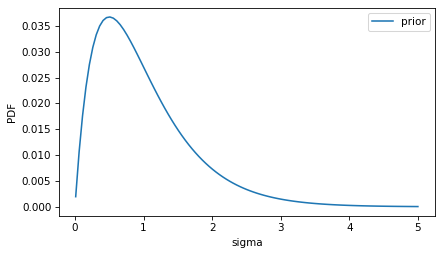
This distribution represents the background knowledge that we expect the standard deviation to be less than 2, and we’d be surprised by anything much higher than that.

I’ll use this function to make a Pandas DataFrame to represent the joint prior.

def make_joint(s1, s2):
    """Compute the outer product of two Series.

    First Series goes across the columns;
    second goes down the rows.

    s1: Series
    s2: Series

    return: DataFrame
    """
    X, Y = np.meshgrid(s1, s2, indexing='ij')
    return pd.DataFrame(X*Y, index=s1.index, columns=s2.index)

prior = make_joint(prior_mu, prior_sigma)
prior.shape

(51, 101)

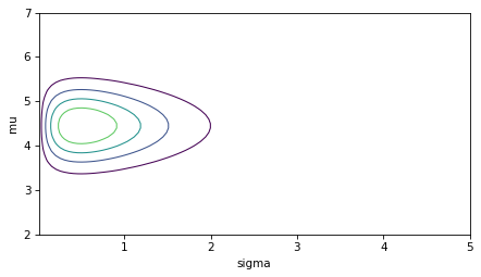
I’ll use the following function to make a contour plot of the prior.

def plot_contour(joint):
    """Plot a joint distribution.

    joint: DataFrame representing a joint PMF
    """
    low = joint.to_numpy().min()
    high = joint.to_numpy().max()
    levels = np.linspace(low, high, 6)
    levels = levels[1:]

    cs = plt.contour(joint.columns, joint.index, joint, levels=levels, linewidths=1)
    decorate(xlabel=joint.columns.name,
             ylabel=joint.index.name)
    return cs

plot_contour(prior)
decorate()

The update

To use the data to update the prior, we have to compute the likelihood of the data for each possible pair of mu and sigma. Can can do that by creating a 3-D mesh with the possible values of mu and sigma, and the observed values of the data.

MU, SIGMA, DATA = np.meshgrid(prior_mu.index, prior_sigma.index, data,
                              indexing='ij')
MU.shape

(51, 101, 6)

Now we can evaluate the normal distribution for each data point and each pair of mu and sigma.

densities = norm(MU, SIGMA).pdf(DATA)
densities.shape

(51, 101, 6)

The likelihood of each pair is the product of the densities for the data points.

likelihood = densities.prod(axis=2)
likelihood.shape

(51, 101)

The unnormalized posterior is the product of the prior and the likelihood.

posterior = prior * likelihood

We can normalize it like this.

def normalize(joint):
    """Normalize a joint distribution.

    joint: DataFrame
    """
    prob_data = joint.to_numpy().sum()
    joint /= prob_data
    return prob_data

normalize(posterior)
posterior.shape

(51, 101)

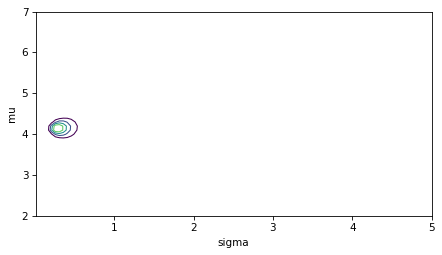
And here’s what the result looks like.

plot_contour(posterior)
decorate()

Here’s the posterior distribution of sigma compared to the prior.

def marginal(joint, axis):
    """Compute a marginal distribution.

    axis=0 returns the marginal distribution of the first variable
    axis=1 returns the marginal distribution of the second variable

    joint: DataFrame representing a joint distribution
    axis: int axis to sum along

    returns: Pmf
    """
    return Pmf(joint.sum(axis=axis))

posterior_sigma = marginal(posterior, 0)

prior_sigma.plot(color='gray', label='prior')
posterior_sigma.plot(label='posterior')

decorate(xlabel='sigma', ylabel='PDF')

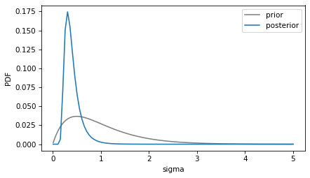
The posterior mean of sigma is about 0.4, somewhat higher than the standard deviation of the data.

posterior_sigma.mean(), np.std(data)

(0.40440859064493323, 0.2687419249432851)

Predictions

The last part of OP’s question is “So, I’m wondering if there’s a way to estimate the range of possibilities of what I would see if I could give 100 or 1000 samples?”

We can simulate a future experiment with larger sample size by drawing random pairs from the joint posterior distribution and generating simulated measurements. That’s easier to do if we stack the posterior PMF.

posterior_pmf = Pmf(posterior.stack())
posterior_pmf.head()

		probs
mu	sigma
2.0	0.0100	0.0
	0.0599	0.0
	0.1098	0.0

Now we can use NumPy’s choice function to choose a random pair of mu and sigma. For each random pair, we can generate 1000 simulated measurements from a normal distribution, and plot the distribution of the results.

for i in range(11):
    mu, sigma = np.random.choice(posterior_pmf.index, p=posterior_pmf)
    sample = np.random.normal(mu, sigma, size=1000)
    sns.kdeplot(sample, alpha=0.3)
    
decorate(xlabel='K+ (mmol/L)')

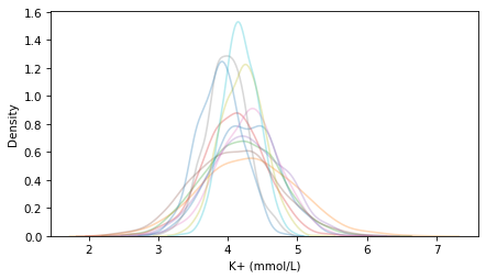
Each line shows the distribution of a possible sample of 1000 measurements. You can see that they vary in both location and spread, due to the uncertainty represented by the posterior distribution of mu and sigma.

Discussion

The normal distribution is probably a good enough model for this data, but for some pairs of mu and sigma in the prior, the normal distribution extends into negative values with non-negligible probability – and for measurements like these, negative values are nonsensical.

An alternative would be to run the whole calculation with the logarithms of the measurements. In effect, this would model the distribution of the data as lognormal, which is generally a good choice for measurements like these.

In this example, the sample size is small, so the choice of the prior is important. I suspect there is more background information we could use to make a better choice for the prior distribution of sigma.

This example demonstrates the use of grid methods for Bayesian statistics. For many common statistical questions, grid methods like this are simple and fast to compute, especially with libraries like NumPy and SciPy. And they make it possible to answer many useful probabilistic questions.

Data Q&A: Answering the real questions with Python

Copyright 2024 Allen B. Downey

License: Creative Commons Attribution-NonCommercial-ShareAlike 4.0 International