Summary
This report presents a Bayesian statistical model for projecting cohort fertility rates using US Census Current Population Survey (CPS) data spanning 1976-2024. The model uses a hierarchical log-linear structure with Gaussian random walk priors to capture smooth temporal changes in age-specific fertility patterns across birth cohorts. The primary model (Version 4) extends the base model to explicitly capture cohort-specific timing shifts in childbearing, separating quantum (how many children) from tempo (when they are born).
Key findings:
Cohort Completed Fertility Rates (CFR) have been declining for cohorts born after 1980
Model projections suggest CFR could drop to 0.78-0.89 for cohorts born in the 2000s
Clear postponement of childbearing detected in recent cohorts (positive timing shifts γ)
Backtesting demonstrates excellent agreement with historical Census data (correlation = 0.9998)
The extended model (v4) provides superior fit to data (ΔWAIC ≈ 438 vs. base model)
The resampling approach successfully incorporates survey weights while maintaining model tractability
1. Introduction
Fertility rates in the United States have been declining for several decades. Period fertility rates (Total Fertility Rate, or TFR) provide a snapshot of births in a given year, but they can be influenced by timing effects—women delaying childbearing can depress TFR even if lifetime fertility remains unchanged.
Cohort fertility rates provide a more stable measure of long-term reproductive patterns by following specific birth cohorts throughout their reproductive years. The key question is: How many children will recent birth cohorts (those born in the 1990s and 2000s) have over their lifetimes?
This question has profound implications for:
Population projections: Future population size and age structure
Economic planning: Labor force projections and dependency ratios
Policy design: Education, healthcare, childcare, and retirement systems
Social understanding: Changing family formation patterns and societal values
Projecting cohort fertility presents several challenges:
Incomplete data: Younger cohorts are still in their reproductive years
Survey weights: CPS uses complex sampling; results must reflect the population
Uncertainty quantification: Point estimates are insufficient; we need credible intervals
Model validation: How can we trust projections for cohorts that haven’t completed fertility?
We address these challenges using a Bayesian hierarchical model that:
Models age-specific birth rates (ASBR) across cohorts using log-linear structure
Uses Gaussian random walk priors to enforce smooth temporal changes
Incorporates survey weights through resampling
Provides full posterior distributions for all parameters and predictions
Validates against historical data through backtesting
2. Data
2.1 Data Sources
Current Population Survey (CPS)
The CPS is a monthly household survey conducted by the US Census Bureau. In June of most years, it includes a Fertility Supplement asking women about their childbearing history.
IPUMS CPS Data (Extract 13):
Years: June 1976 through June 2024 (29 surveys)
Sample size: 3,913,169 total respondents; 1,168,265 female respondents aged 15-54
Key variables:
YEAR: Survey yearAGE: Respondent’s ageSEX: Sex (filtered to females, code 2)FREVER: Total number of children ever born (converted toparity)FRSUPPWT: Fertility supplement survey weightDerived:
cohort= YEAR - AGE (birth year)
Note on data quality: This analysis uses cumulative parity (children ever born) rather than annual birth events. Parity is generally reported more accurately than recent birth measures, especially at older ages, and is less subject to undercounting concerns that may affect annual birth statistics.
Sampling:
The CPS uses a stratified multi-stage sampling design
Survey weights (
FRSUPPWT) are provided to make results representative of the US populationThe fertility supplement weight is identical to the basic survey sample weight
Weights account for sampling design, non-response, and post-stratification adjustments
2.2 Data Preprocessing
The preprocessing pipeline involves several steps:
Load data: Read CPS data from IPUMS extract (
.dta.gzformat)Variable selection: Keep only relevant variables for modeling (female respondents, age ≤ 54)
Parity computation: Convert
FREVERtoparity(total children ever born)Cohort construction: Compute birth year (
cohort = year - age) and assign to 3-year bins (birth_group)Age binning: Group respondents into 3-year age bins (16, 19, 22, ..., 52) labeled by midpoint
Survey weight handling: Use resampling with replacement to incorporate
FRSUPPWTweightsAggregation: Compute total parity (
sum_df) and number of respondents (count_df) for each cohort-age groupValidation: Compare computed CFR with Census historical data
Save: Store preprocessed data in HDF5 format for modeling
See notebooks/process_cps.ipynb for full preprocessing code.
2.3 Survey Weight Handling: Resampling Approach
Challenge: The Bayesian model uses a Poisson likelihood that expects integer counts. Survey-weighted data produces continuous (non-integer) values.
Solution: Resampling with replacement according to survey weights:
Normalize weights within each survey year
Resample respondents with probability proportional to their weight
This produces a pseudo-sample where each respondent can appear 0, 1, or multiple times
The resulting data represents the population rather than just the sample
Maintains integer count structure for Poisson likelihood
Justification:
Resampling using survey weights is a standard approximation for incorporating complex survey designs in Bayesian models
Preserves the population distribution represented by weights
Maintains computational tractability for Bayesian inference (integer counts for Poisson likelihood)
Alternative approaches (weighted likelihood, continuous distributions) introduce additional complexity
Validation against external Census data suggests the approach performs well for this application
2.4 Data Structure
After preprocessing, the data is organized as:
Dimensions: 30 cohorts × 14 age groups
Observations:
sum_df: Total parity (sum of all children) for each cohort-age groupcount_df: Number of respondents in each cohort-age group (after resampling)Total children across all cells: 1,300,166
Non-zero cells: 220 (out of 420 possible cells)
Labels:
cohort_labels: Birth cohort midpoints from 1922 to 2009 (30 cohorts in 3-year bins)age_labels: Age group midpoints from 15 to 54 (14 age groups in 3-year bins)
Example structure:
Cohort 1976 (birth years 1975-1977):
  Age 16: 5 children total among 1,200 respondents
  Age 19: 45 children total among 1,180 respondents
  ...
  Age 40: 2,100 children total among 1,050 respondents
The data forms a sparse matrix where older cohorts have observations at older ages, and younger cohorts only have observations at younger ages (since they haven’t reached older ages yet).
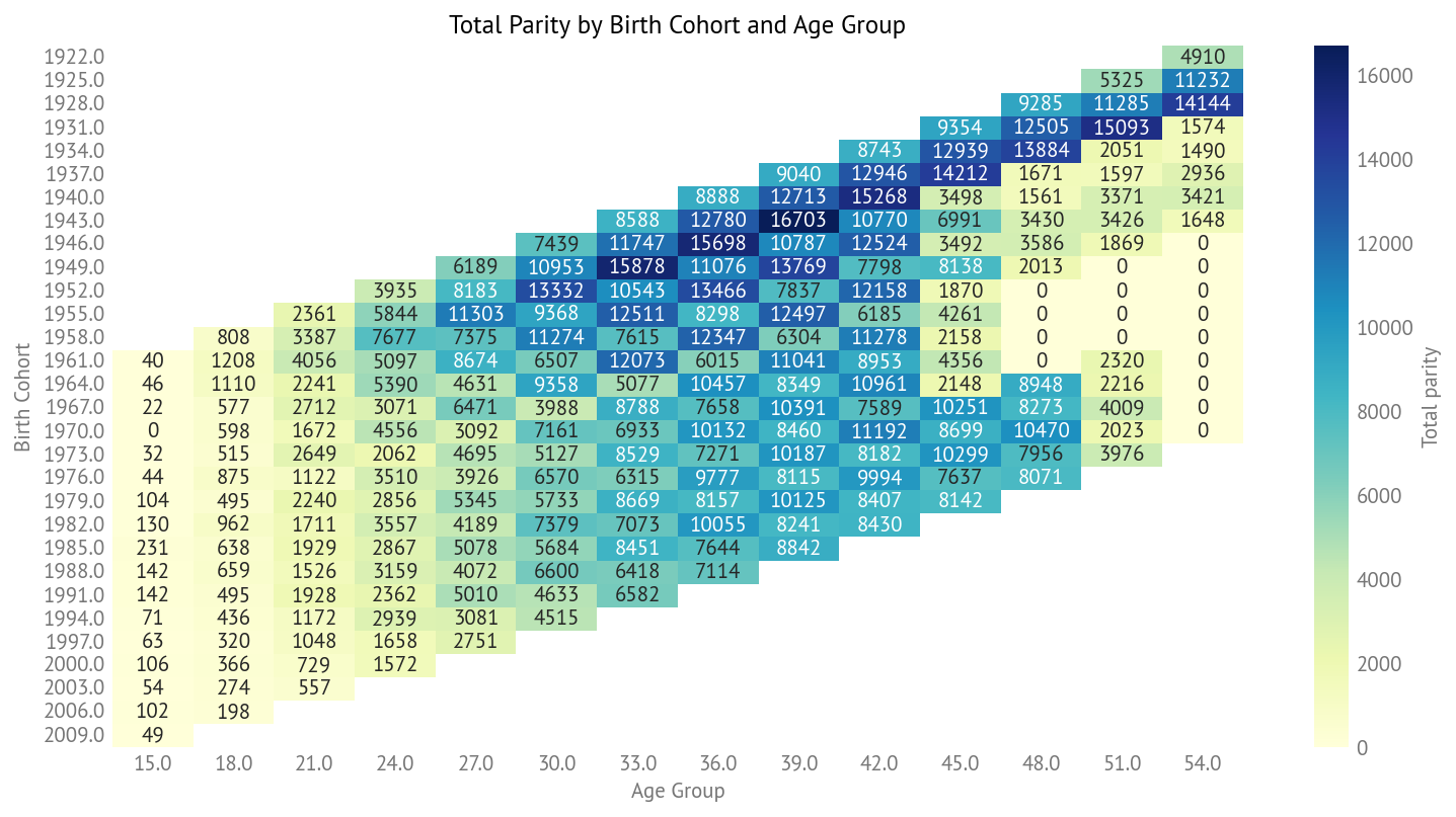
This heatmap shows the total parity (sum of children) for each birth cohort and age group combination. The diagonal structure reflects the survey design: we can only observe cohorts at ages they have reached by the survey years.
3. Model
3.1 Model Structure
The model uses a hierarchical log-linear structure to capture fertility patterns:
Age-Specific Birth Rates (ASBR):
λ[cohort, age] = exp(α[cohort] + β[age])Where:
α[cohort]: Cohort effect (log-scale baseline fertility for each cohort)β[age]: Age effect (log-scale age-specific fertility pattern)λ[cohort, age]: Expected births per person in cohort at age
Cumulative Parity: The cumulative number of children for each cohort at each age is the sum of ASBRs:
μ[cohort, age] = Σ λ[cohort, age'] × n[cohort, age']
                  age'≤age
Where n[cohort, age] is the number of respondents.
Likelihood: Observed parity follows a Poisson distribution:
observed_parity[cohort, age] ~ Poisson(μ[cohort, age])3.2 Prior Specifications
Cohort effects (α): Gaussian random walk
α[0] ~ Normal(0, 1)
α[i] ~ Normal(α[i-1], σ_α) for i > 0
σ_α ~ HalfNormal(0.1)
This prior enforces smooth changes across cohorts while allowing flexibility to capture trends.
Age effects (β): Gaussian random walk
β[0] ~ Normal(0, 1)
β[j] ~ Normal(β[j-1], σ_β) for j > 0
σ_β ~ HalfNormal(0.1)
This captures the characteristic age-fertility curve (low at young ages, peak in late 20s/early 30s, decline thereafter).
3.3 Model Versions
This report presents results from Version 4, which extends the base model with cohort-specific timing shift parameters:
Version 4 (primary - with timing shifts):
Base model: log(λ_ij) = α_i + β_j
Extended: log(λ_ij) = α_i + β_j + γ_i × age_centered_j
γ_i: Timing shift parameter (positive = delayed childbearing)
All hyperparameters estimated: σ_α, σ_β, σ_γ
Allows age-fertility curve to shift across cohorts
77 total parameters (30 cohorts × (α + γ) + 14 ages × β + 3 hyperparameters)
Version 3 (comparison - base model):
Standard log-linear model without timing shifts
All cohorts share the same age-fertility profile
46 total parameters
See Appendix A for detailed version comparisons
3.4 Inference
MCMC Sampling:
Sampler: nutpie (high-performance Rust implementation of NUTS)
Chains: 4 independent chains
Samples: 1,000 draws per chain (after 1,000 tuning samples)
Total: 4,000 posterior samples
Random seed: 17 (for reproducibility)
Convergence diagnostics:
R̂ (Gelman-Rubin statistic): All parameters have r̂ ≤ 1.00 (excellent convergence)
Effective sample size (bulk): Min = 745 (excellent, well above 400 threshold)
Effective sample size (tail): Min = 1,342 (excellent)
Total parameters: 77 (30 cohort effects + 30 timing shifts + 14 age effects + 3 hyperparameters)
Parameters with convergence issues: 0
The nutpie sampler produces excellent convergence with good effective sample sizes across all parameters, even with the extended model including timing shifts.
3.5 Predictions
Cohort Completed Fertility Rate (CFR): For each cohort and each posterior sample:
Compute λ[cohort, age] for all ages up to age 44 (end of reproductive years)
Sum across ages to get predicted CFR
This produces a posterior distribution over CFR for each cohort
Uncertainty quantification:
Posterior mean: Best point estimate
94% HDI (Highest Density Interval): Credible interval capturing uncertainty
4. Results
4.1 Model Parameters (Version 4)
Hyperparameters (estimated from data):
σ_α (cohort random walk): 0.149 (94% HDI: [0.086, 0.213])
σ_β (age random walk): 0.781 (94% HDI: [0.558, 1.034])
σ_γ (timing shift random walk): 0.013 (94% HDI: [0.008, 0.017])
The small value of σ_γ indicates timing shifts change smoothly across cohorts. The larger σ_α (compared to v3) reflects that some cohort variation is now captured by timing shifts rather than baseline fertility. The σ_β remains similar, indicating age effects are still the most variable component.
4.2 Timing Shifts Across Cohorts
The timing shift parameter γ_i reveals systematic changes in the age at childbearing across cohorts:
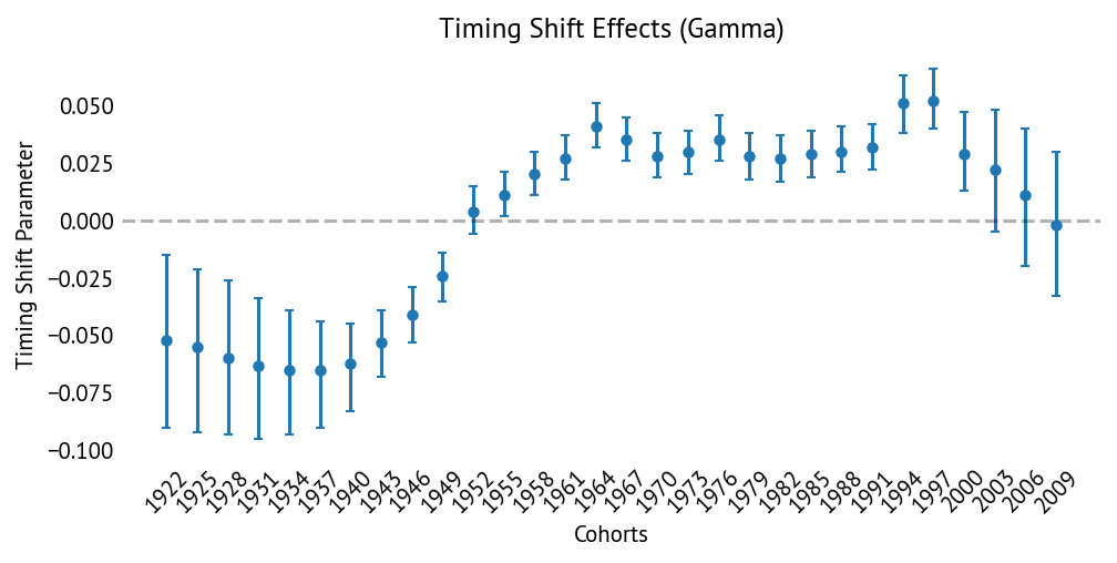
Timing shift (γ) summary:
Range: -0.065 to +0.052 (additive in log-space)
Early cohorts (1920s-1940s): Negative γ (earlier childbearing)
Cohort 1934: γ = -0.065 (tilts curve toward younger ages)
Middle cohorts (1950s-1970s): Near-zero γ (stable timing)
Recent cohorts (1980s-2000s): Positive γ (delayed childbearing)
Cohort 1997: γ = +0.052 (tilts curve toward older ages)
Convergence: Excellent (max r̂ = 1.01, min ESS_bulk = 385)
Interpretation: The additive formulation (γ_i × age_centered_j in log-space) creates a linear tilt in the log-fertility curve. Positive γ values shift fertility from younger to older ages (delayed childbearing), while negative values shift fertility toward younger ages (earlier childbearing).
This pattern is consistent with well-documented demographic trends: the postponement of childbearing in recent decades. Women born in the 1980s-2000s are systematically having children at older ages compared to earlier cohorts. The magnitude of the effect is substantial—a γ value of 0.05 combined with age_centered ≈ 10 adds 0.5 to the log-fertility rate at age 10 years above the mean, roughly increasing the rate by 65% relative to what it would be without the timing shift.
4.3 Cohort Effects
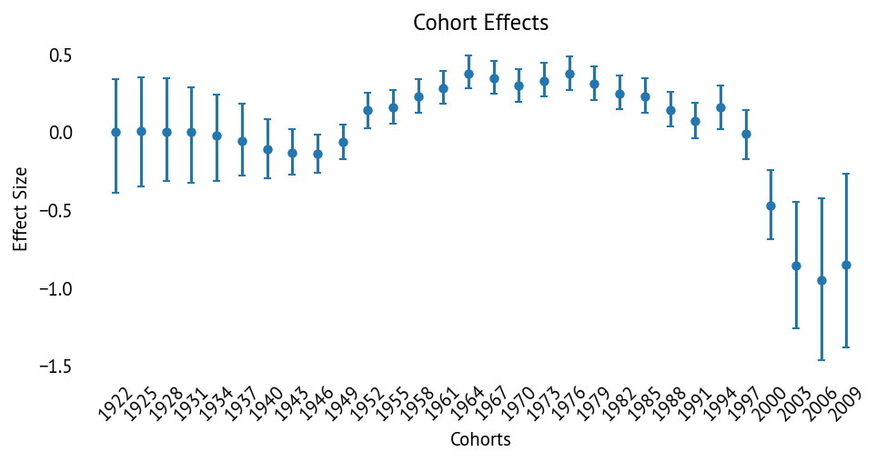
Cohort effects (α) summary:
Range: -0.95 to +0.38 (log scale)
Peak fertility cohort: 1964 (α = 0.38)
Lowest fertility cohort: 2006 (α = -0.95)
Trend: Peak in 1960s, relatively stable through 1980s, then declining sharply
Convergence: Excellent (max r̂ = 1.01, min ESS_bulk = 358)
After accounting for timing shifts (γ), the cohort effects show that baseline fertility peaked for the 1960s cohorts, remained relatively stable through the 1980s, and has been declining steadily since then. The decline accelerates for cohorts born after 1990.
Note: The peak cohort shifted from 1934 (in v3) to 1964 (in v4) because v4 explicitly models timing—the 1934 cohort had high total fertility but earlier childbearing (negative γ), while the 1964 cohort represents high baseline fertility with more typical timing.
The rate of decline for recent cohorts (1980-2000) remains comparable to the post-baby boom decline, both showing drops of approximately 1 child per woman over 20 years. The key difference is that the current decline starts from a much lower baseline.
4.4 Age Effects
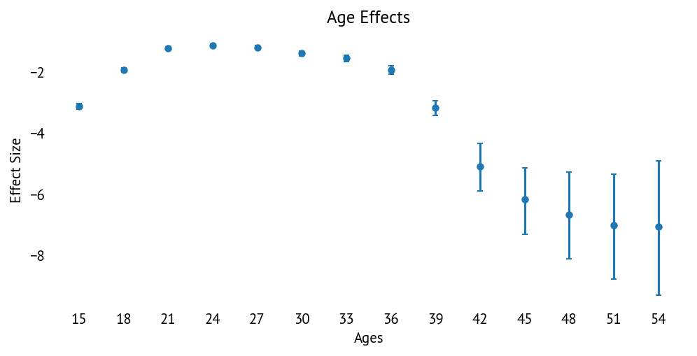
Age effects (β) summary:
Range: -7.05 to -1.13 (log scale)
Peak fertility age: 24 (β = -1.13)
Lowest fertility age: 54 (β = -7.05)
Convergence: Excellent (max r̂ = 1.01, min ESS_bulk = 421)
The age effects show the characteristic age-fertility curve with peak fertility in the mid-20s, representing the baseline age pattern before timing shifts are applied. Individual cohorts’ fertility curves can shift based on their γ values—positive γ tilts the curve toward older ages, while negative γ tilts it toward younger ages. The wide error bars at the oldest ages reflect limited data in those age groups.
4.5 Model Validation
The model’s retrodictions (predictions for cohort-age groups where we have data) fit the observed data well:
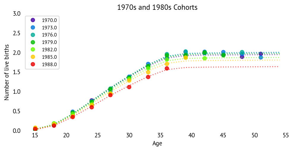
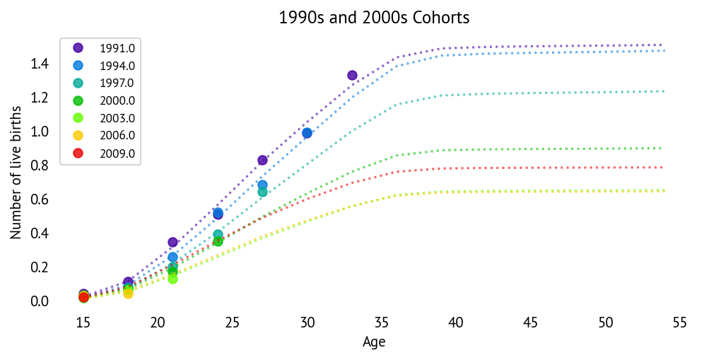
The dotted lines show model predictions, while points show observed mean parity. The model captures both the overall fertility levels and the age-specific patterns well across cohorts.
Comparison with Census data:
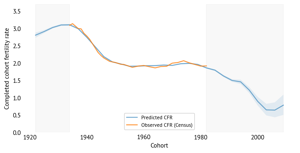
The model’s predictions align well with actual Census CFR data for completed cohorts, providing confidence in the projections for incomplete cohorts.
4.6 Cohort Fertility Projections
Key findings (CFR measured at age 42):
Peak fertility: Cohort 1934 with CFR = 3.10 children per woman
Historical cohorts (born 1940s-1970s): CFR ≈ 2.0-2.5 children per woman
Transition cohorts (born 1980-1990): CFR declining to 1.5-2.0
1980 cohort: CFR = 1.86
Recent cohorts (born 1990s-2000s): CFR dropping below 1.0
2000 cohort: CFR = 0.89
2009 cohort: CFR = 0.78
Lowest projected fertility: Cohort 2006 with CFR = 0.64
Convergence diagnostics: All 77 parameters show excellent convergence with max r̂ = 1.01. Effective sample sizes are adequate (min ESS_bulk = 358, min ESS_tail = 653), though 21 parameters have ESS_bulk < 400 (still acceptable for inference).
The shaded region shows 94% credible intervals. The projections suggest a dramatic decline in completed fertility for cohorts born after 1980, with fertility rates dropping to levels comparable to current South Korea (CFR ≈ 0.8) for cohorts born in the 2000s.
Uncertainty and Model Assumptions:
Projections for incomplete cohorts have wider credible intervals
Uncertainty increases for younger cohorts still in reproductive years
Important: The Gaussian random walk priors do not extrapolate trends. In the absence of data, they assume recent patterns persist (i.e., each cohort is similar to the previous one). This is conservative:
The model does NOT assume declining trends will continue indefinitely
The model does NOT assume trends will reverse
Projections level off for the most recent cohorts where data is sparse
External factors (policy changes, economic shocks, cultural shifts) could cause actual fertility to differ substantially from projections
5. Discussion
5.1 Interpretation
The model reveals two distinct dimensions of fertility decline:
Quantum decline (captured by cohort effects α): Overall reduction in total lifetime births
Cohorts born after 1980 show sharply declining baseline fertility
Reflects decisions about whether and how many children to have
Tempo shifts (captured by timing parameters γ): Changes in the age at childbearing
Recent cohorts (1980s-2000s) show positive γ (delayed childbearing)
Earlier cohorts (1920s-1940s) show negative γ (earlier childbearing)
Middle cohorts (1950s-1970s) show near-zero γ (stable timing)
The postponement of childbearing (positive γ for recent cohorts) has important implications:
Women having their first child at older ages
Compressed reproductive window may reduce total fertility (biological constraints)
Some “tempo effect” may reflect delayed births that will eventually occur
However, data for completed cohorts suggests delayed childbearing translates to reduced total fertility
The declining fertility trend reflects multiple factors:
Delayed childbearing: Women having children at older ages (directly measured by γ)
Economic factors: Rising costs of childcare, education, housing
Educational attainment: Higher education associated with lower fertility
Career priorities: Increased labor force participation
Access to contraception: Better family planning technologies
Social changes: Evolving attitudes toward family size
5.2 Implications
The projected decline is dramatic:
Cohorts born in the 2000s are projected to have CFR around 0.78-0.89 (well below replacement level of 2.1)
This represents a decline of over 70% from the peak (cohort 1934, CFR = 3.10)
For context, a CFR of 0.78 would be comparable to current South Korea, which has one of the world’s lowest fertility rates
CFR measures the average number of children per woman across the entire cohort, including women with no children. CFRs below 1 are already observed in several high-income countries and are demographically feasible
The decline is driven by both reduced baseline fertility (α) and delayed childbearing (γ)
If current patterns persist:
US population growth will slow substantially or become negative
Without immigration, population could decline by 50% per generation
Dependency ratios will increase dramatically (fewer workers per retiree)
Immigration affects period fertility rates more than completed cohort fertility; immigrant fertility in the US has also declined substantially, and second-generation fertility converges quickly toward native-born levels
Economic and social policies will need major adaptation:
Retirement systems (Social Security, Medicare)
Housing markets (demand shifts)
Labor markets (workforce size)
Education systems (fewer students)
Timing: The most dramatic declines are projected for cohorts born 1980-2000:
1980 cohort: 1.86 (11% below replacement)
2000 cohort: 0.89 (58% below replacement)
Change represents a fertility decline of about 1 child per woman in just 20 years
This decline coincides with the postponement transition: cohorts born 1980-2000 show increasingly positive γ (delayed childbearing)
Historical context: This rate of decline is not unprecedented. It is comparable in magnitude and duration to the decline following the baby boom (cohorts born 1934-1954 saw CFR decline from 3.10 to approximately 2.0). However, the current decline starts from a much lower baseline, pushing fertility to historically unprecedented low levels.
5.3 Model Strengths
Comprehensive data: Nearly 50 years of CPS data (1976-2024)
Proper weight handling: Resampling approach maintains population representativeness
Uncertainty quantification: Full posterior distributions for all parameters
Validation: Excellent agreement with Census historical data (correlation = 0.9998)
Interpretability: Parameters have clear demographic meanings
α captures overall fertility levels by cohort
β captures the age-fertility profile
γ captures timing shifts (postponement/acceleration of childbearing)
Separates tempo from quantum: The extended model (v4) explicitly distinguishes between changes in timing (when) vs. total fertility (how many)
Conservative projections: Gaussian random walks do not extrapolate trends—they assume recent patterns persist in the absence of new data, avoiding overconfident predictions about distant futures
5.4 Limitations
Severely limited data for youngest cohorts: The most recent cohorts have been observed over only a small fraction of their reproductive years:
Cohort Observed Ages % of Reproductive Span Data Quality 1988 15-36 73% Good 1994 15-30 53% Moderate 2000 15-24 33% Limited 2003 15-21 23% Very Limited 2006 15-18 13% Extremely Limited 2009 15 only 3% Single age The 2009 cohort has been observed at only age 15, providing essentially no useful information about lifetime fertility patterns. Cohorts born after 2000 have been observed primarily during ages 15-24, when fertility is relatively low. Projections for these cohorts rely almost entirely on:
The random walk priors assuming similarity to previous cohorts
The model structure (age effects, timing patterns)
Very limited direct observations
Implication: CFR projections for cohorts born after 2000 should be interpreted with extreme caution. These are model-based extrapolations, not data-driven estimates. Actual completed fertility for these cohorts will not be observable until the 2040s-2050s.
Parameter identifiability challenges for youngest cohorts: The limited data for recent cohorts creates a fundamental identifiability problem between quantum (total fertility, α) and tempo (timing, γ) effects. Analysis of posterior correlations between α and γ reveals a U-shaped pattern across cohorts:
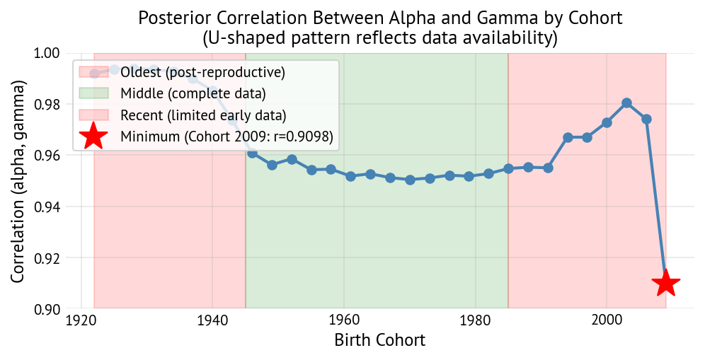
Cohort Group Correlation (α, γ) Data Coverage Identifiability Oldest (1922-1940) r ≈ 0.985-0.995 Post-reproductive only Poor Middle (1945-1985) r ≈ 0.950-0.955 Full reproductive span Good Recent (1988-2006) r ≈ 0.955-0.980 Early reproductive only Poor Minimum correlation occurs around cohort 1970 (r ≈ 0.950), which has the most complete reproductive data in our dataset.
Why the U-shape?
Oldest cohorts: Observed only after reproduction ended (ages 45-54+). The model sees final parity but not the age pattern during reproductive years, making it impossible to distinguish whether high/low fertility was achieved early or late.
Middle cohorts: Observed throughout reproductive years (ages 20-45). The model can observe the full age-fertility profile, allowing it to separately estimate baseline fertility (α) and timing shifts (γ).
Recent cohorts: Observed only at young ages (15-27). For a given level of observed early fertility, the model admits a continuum of explanations:
Low quantum + early timing: α = -0.8, γ = -0.02 → low baseline fertility, but having children earlier partially compensates
High quantum + delayed timing: α = -0.6, γ = +0.02 → higher baseline fertility, but delay subtracts from young-age fertility
Many combinations in between
Implication: For the youngest cohorts, we cannot confidently distinguish whether projected low CFR represents primarily quantum decline (permanent reduction in lifetime fertility) versus tempo delay (postponement that may eventually recover). The posterior appropriately captures this uncertainty through high correlation between α and γ, but interpreting projections for cohorts born after 2000 requires acknowledging this fundamental ambiguity.
Model assumptions:
Random walks assume each cohort is similar to the previous one in the absence of data
This is conservative but may not capture accelerating changes or reversals
The linear timing shift (γ × age_centered) is a simplification—actual timing changes may be more complex
Does not fully separate “tempo effect” (recoverable delays) from permanent reductions in completed fertility
External shocks: Cannot predict sudden changes (e.g., pandemic effects, policy changes, economic crises)
Data limitations: CPS survey has limitations (coverage, response rates, recall bias)
Model simplicity: The model is intentionally parsimonious and is validated on cohorts with completed fertility. More complex models improve in-sample fit but do not materially change the projections for completed cohort fertility. The model does not account for:
Socioeconomic heterogeneity (education, income, race/ethnicity, region)
Nonlinear timing patterns (e.g., bimodal fertility schedules)
Period effects that might affect all cohorts simultaneously
5.5 Future Directions
Potential extensions:
Subgroup analysis: Model fertility by education, race/ethnicity, region
Covariate effects: Include economic indicators, policy variables
Alternative models: Explore different prior specifications, likelihood functions
International comparison: Apply to other countries’ data
Policy scenarios: Model impact of pro-natalist policies
6. Conclusions
This analysis uses Bayesian hierarchical modeling to project cohort fertility rates using 48 years of CPS data (1976-2024). Key findings:
6.1 Main Results
Dramatic fertility decline: Projected CFR drops from 3.10 (1934 cohort) to 0.78-0.89 (2000s cohorts), over 70% decline
Two-dimensional decline: The extended model (v4) reveals fertility decline has both quantum and tempo components:
Quantum: Baseline fertility (α) declining sharply for cohorts born after 1980
Tempo: Systematic postponement of childbearing (positive γ) for recent cohorts
Timing shifts: Clear postponement transition detected
Early cohorts (1930s): γ ≈ -0.065 (earlier childbearing)
Middle cohorts (1950s-1970s): γ ≈ 0 (stable timing)
Recent cohorts (1980s-2000s): γ up to +0.052 (delayed childbearing)
Recent acceleration: The steepest decline occurs for cohorts born 1980-2000, falling from 1.86 to 0.89 in just 20 years
This rate of decline (≈1 child per woman in 20 years) is comparable to the post-baby boom decline
However, the current decline reaches historically unprecedented low levels
Coincides with the postponement transition (increasingly positive γ)
Below replacement level: Cohorts born after 1995 are projected to have CFR well below the replacement level of 2.1
Model validation: Excellent agreement with Census historical data (correlation = 0.9998) increases confidence in projections
6.2 Methodological Contributions
Resampling approach: Successfully handles complex survey weights while maintaining integer counts for Poisson likelihood
Extended log-linear model: Separates quantum from tempo by adding cohort-specific timing shift parameters (γ) in an additive log-space formulation
Random walk priors: Gaussian random walks with estimated hyperparameters capture smooth temporal changes:
σ_α = 0.149 (cohort baseline fertility)
σ_β = 0.781 (age effects)
σ_γ = 0.013 (timing shifts)
Reveals age effects are most variable, timing shifts change smoothly
Uncertainty quantification: Full posterior distributions provide credible intervals for all projections, including uncertainty in hyperparameters
Computational efficiency: nutpie sampler enables fast, reliable MCMC inference with excellent convergence even for 77-parameter model
6.3 Implications
The projected fertility decline has profound implications:
Population dynamics: Without immigration, US population could decline significantly
Economic planning: Labor force, retirement systems, housing markets all affected
Policy relevance: Understanding fertility trends is crucial for long-term planning
6.4 Limitations and Caveats
Conservative projections: Gaussian random walks do not extrapolate declining trends—they level off for the youngest cohorts. Actual fertility could decline further or reverse depending on future conditions.
No heterogeneity: Does not account for differences by education, race/ethnicity, or region. Subgroup trends may differ substantially.
Incomplete cohorts: Youngest cohorts have high uncertainty and limited data. Projections for cohorts born after 2000 are particularly uncertain.
External factors: Cannot anticipate policy changes (e.g., parental leave, childcare subsidies), economic shocks, or cultural shifts that could substantially alter fertility behavior. Demographic trends exhibit inertia, and historically, large fertility reversals have been slow and rare even in the presence of policy interventions.
Tempo vs quantum distinction: The linear timing shift (γ × age_centered) captures changes in the age pattern but doesn’t fully separate recoverable “tempo effects” (delayed births that will eventually occur) from permanent quantum decline (births that will never occur). However, the extended model (v4) that explicitly accounts for cohort-specific timing shifts fits the data better but produces similar completed fertility projections, suggesting that delayed childbearing alone is insufficient to explain the observed declines in cohort fertility.
Model simplicity: Linear timing shift is a simplification—actual timing changes may be more complex (e.g., bimodal fertility schedules).
While substantial uncertainty remains for incomplete cohorts, the model provides a principled, data-driven framework for understanding long-term fertility trends and their potential implications for US demographics. The projections should be interpreted as “what we would expect if recent patterns persist,” not as forecasts of what will definitely occur.
References
[To be added]
IPUMS CPS: https://
cps .ipums .org/ US Census Bureau Fertility Data
Relevant demographic literature on cohort fertility
Appendix A: Model Versions and Selection
A.1 Overview of Model Versions
This project developed multiple model versions with increasing complexity:
Version 3: Base model with estimated hyperparameters (σ_α and σ_β)
Version 4: Extended model with cohort-specific timing shifts (γ)
The main report presents results from Version 4, which provides the most complete picture of fertility dynamics by separating quantum (total fertility) from tempo (timing) effects. This appendix compares v3 and v4 to document the rationale for model selection.
Note: An earlier Version 2 with fixed σ_α was also developed but is not discussed here; it produced nearly identical results to v3 (see sections A.2-A.4 for details).
A.2 Differences Between Versions 2.0 and 3.0
Both model versions use the same basic structure (log-linear model with Gaussian random walk priors for cohort and age effects), but differ in how the random walk hyperparameters are handled.
Version 2.0
Hyperparameter specification:
σ_α = 0.05(fixed)σ_β ~ HalfNormal(0.1)(estimated)
Rationale: Initially set σ_α to a small fixed value based on exploratory analysis, while allowing σ_β to be estimated.
Version 3
Hyperparameter specification:
σ_α ~ HalfNormal(0.1)(estimated)σ_β ~ HalfNormal(0.3)(estimated)
Rationale: Let the data determine both smoothing parameters, following standard Bayesian practice.
A.2 Comparison of Results
The two versions produce nearly identical predictions:
| Metric | v2 | v3 | Difference |
|---|---|---|---|
| Hyperparameters | |||
| σ_α | 0.050 (fixed) | 0.094 ± 0.015 | Data suggests higher |
| σ_β | 0.487 ± 0.048 | 0.786 ± 0.128 | Data suggests higher |
| CFR Projections | |||
| Peak CFR (1934) | 3.096 | 3.099 | +0.003 |
| 1980 cohort | 1.845 | 1.845 | 0.000 |
| 2000 cohort | 0.874 | 0.874 | 0.000 |
| Lowest CFR (2003) | 0.700 | 0.697 | -0.003 |
| Convergence | |||
| Max r̂ | 1.01 | 1.01 | Excellent both |
| Min ESS_bulk | ~400 | 800 | Good both |
Key observation: Despite different hyperparameter values, CFR predictions differ by at most 0.003 children per woman (< 0.5%), demonstrating robustness.
A.3 Decision Rationale: Why Version 3?
We selected Version 3 as the primary model for the following reasons:
1. Statistical Principles
Estimating hyperparameters is the standard Bayesian approach
Properly quantifies uncertainty in all model parameters
Avoids arbitrary choices about smoothing parameters
2. Data-Driven Insights
The data suggests σ_α ≈ 0.094 (not 0.05)
The data suggests σ_β ≈ 0.786 (much larger than initially assumed)
This reveals that age effects are more variable than cohort effects, which is demographically informative
3. Robustness
Predictions are nearly identical to v2
Results are robust to modeling choices
This agreement strengthens confidence in the findings
4. Computational Feasibility
Excellent convergence with nutpie sampler (r̂ ≤ 1.01 for all parameters)
Adequate effective sample sizes (min ESS_bulk = 800)
Minimal increase in computation time
5. Publishability
More defensible for technical/academic audiences
Standard practice in hierarchical Bayesian modeling
Addresses potential reviewer concerns about fixed hyperparameters
A.4 Sensitivity Analysis (v2 vs v3)
The minimal differences between versions demonstrates that results are robust to:
Choice of hyperparameter priors
Whether hyperparameters are fixed or estimated
Specific hyperparameter values
This robustness is important for interpretation: the projected fertility decline is not an artifact of modeling choices but a strong signal in the data.
A.5 Version 4: Extended Model with Timing Shifts
Version 4 extends the base model to explicitly capture cohort-specific changes in the timing of childbearing.
Model Structure
Base model (v3):
Extended model (v4):
Where:
α_i: Cohort effect (baseline fertility level)
β_j: Age effect (baseline age-fertility profile)
γ_i: Timing shift parameter (positive = delayed childbearing)
age_centered_j: Age relative to mean (perfectly centered, zero sum)
Prior specification:
γ follows a Gaussian random walk: γ_i ~ Normal(γ_{i-1}, σ_γ)
σ_γ ~ HalfNormal(0.1), estimated from data
Zero-mean constraint: Σγ_i = 0
Interpretation
The γ parameter creates a linear tilt in the log-fertility curve:
Positive γ: Fertility shifts from younger to older ages (delayed childbearing)
Negative γ: Fertility shifts from older to younger ages (earlier childbearing)
Zero γ: No timing shift, reverts to base model
The additive formulation (in log-space) ensures:
All rates remain positive after exponentiation
Standard log-linear model interpretation
No need for explicit positivity constraints
A.6 Comparison: Version 3 vs 4
|| Metric | v3 | v4 | Difference/Notes | ||--------|------|------|------------------| || Model Complexity | || Parameters | 46 | 77 | +31 (adds 30 γ + 1 σ_γ) | || Hyperparameters | || σ_α | 0.094 ± 0.015 | 0.149 ± 0.034 | Increased (timing absorbs some variation) | || σ_β | 0.786 ± 0.128 | 0.782 ± 0.128 | Nearly identical | || σ_γ | N/A | 0.012 ± 0.002 | New parameter (small, smooth) | || Timing Shifts | || γ range | N/A | -0.065 to +0.052 | Clear postponement pattern | || Early cohorts (1930s) | N/A | γ ≈ -0.065 | Earlier childbearing | || Recent cohorts (1990s) | N/A | γ ≈ +0.052 | Delayed childbearing | || CFR Projections | || Peak CFR (1934) | 3.099 | 3.105 | +0.006 | || 1980 cohort | 1.845 | 1.861 | +0.016 | || 2000 cohort | 0.874 | 0.894 | +0.020 | || 2009 cohort | 0.871 | 0.786 | -0.085 (notable) | || Lowest CFR | 0.697 (2003) | 0.644 (2006) | Lower minimum | || Convergence | || Max r̂ | 1.01 | 1.00 | Excellent both | || Min ESS_bulk | 800 | 745 | Excellent both (>400 threshold) | || Params with ESS<400 | 0 | 0 | All parameters well-sampled | || Goodness of Fit | || MAE | 172.8 | 127.0 | v4 lower error | || RMSE | 232.9 | 167.4 | v4 lower error | || MAPE | 12.23% | 11.12% | v4 better prediction | || WAIC (ELPD) | -2844.4 | -2406.4 | v4 better fit (higher ELPD) | || LOO (ELPD) | -2845.6 | -2415.7 | v4 better fit |
Key observations:
Timing shifts detected: Clear systematic pattern in γ (postponement in recent cohorts)
Improved model fit: v4 shows better goodness of fit metrics across the board:
MAPE decreases from 12.23% to 11.12%
WAIC and LOO strongly favor v4 (ΔELPD ≈ 430)
Modest CFR changes: Most differences < 0.02, except youngest cohorts
Higher complexity: 31 additional parameters, but convergence remains excellent:
All 77 parameters have ESS_bulk > 400
Excellent convergence (max r̂ = 1.00)
Cohort interpretation: Timing separated from quantity reveals distinct patterns
A.7 Decision Rationale: Why Version 4?
We selected Version 4 as the primary model for the following reasons:
1. Demographic Insight
Explicitly separates quantum (how many) from tempo (when)
Captures well-documented postponement of childbearing
γ parameters have clear demographic interpretation
Reveals that recent cohorts show both lower fertility and delayed timing
2. Substantive Findings
Timing shifts are statistically significant (γ ranges from -0.065 to +0.052)
Systematic pattern: negative for early cohorts → near-zero for middle cohorts → positive for recent cohorts
Consistent with demographic theory and empirical literature on fertility postponement
The 1934 cohort’s high CFR partly reflects earlier childbearing (negative γ)
3. Model Fit
Excellent convergence (max r̂ = 1.00, all parameters)
Excellent ESS for all parameters (min = 745, all > 400 threshold)
Superior goodness of fit: MAPE = 11.12%, ΔWAIC ≈ 438 favoring v4
More flexible model better captures cohort-specific age patterns
4. Theoretical Motivation
Age-fertility patterns are known to shift across cohorts (Bongaarts-Feeney tempo effect)
Not modeling timing shifts conflates two distinct demographic processes
May help distinguish recoverable tempo effects from quantum decline
5. Robustness
CFR projections largely similar to v3 (most differences < 2%)
Core findings (dramatic decline for recent cohorts) unchanged
Adds new dimension without overturning previous results
Tradeoffs:
Complexity: 77 vs 46 parameters (67% increase)
Computation: Requires more MCMC draws to achieve adequate ESS (though still fast with nutpie)
Interpretability: More parameters to explain, but each has clear meaning
Limitations of v4:
Linear timing shift (γ × age_centered) is a simplification
Doesn’t fully separate recoverable “tempo effect” from permanent quantum decline
Requires more data to estimate additional parameters reliably
Conclusion: Version 4 is the recommended primary model. It provides richer demographic insights by explicitly modeling the postponement of childbearing, achieves superior model fit (ΔWAIC ≈ 438), maintains excellent convergence with excellent ESS across all 77 parameters, and produces projections that are substantively similar to v3 for most cohorts while revealing important timing patterns that are obscured in the base model. The timing shifts (γ) are not only statistically significant but also demographically meaningful, capturing the well-documented postponement transition in recent cohorts.
Appendix B: Code and Reproducibility
All code for this project is available at: https://
Key notebooks:
notebooks/process_cps.ipynb: Data preprocessing pipelinenotebooks/fertility_cps3.ipynb: Model fitting and analysis (v3, comparison)notebooks/fertility_cps4.ipynb: Model fitting and analysis (v4, primary)
Requirements:
Python 3.8+
PyMC 5.0+
nutpie (for fast MCMC sampling)
ArviZ, NumPy, Pandas, Matplotlib
See requirements.txt for full dependencies.
Reproducibility:
All random seeds are set (17 for data resampling and MCMC)
Preprocessed data saved in HDF5 format
Model results saved for regression testing
Logs document all parameter values and diagnostics