3. Proper Motion
In the previous lesson, we wrote a query to select stars from the region of the sky where we expect GD-1 to be, and saved the results in a FITS file.
Now we’ll read that data back and implement the next step in the analysis, identifying stars with the proper motion we expect for GD-1.
Outline
Here are the steps in this lesson:
We’ll read back the results from the previous lesson, which we saved in a FITS file.
Then we’ll transform the coordinates and proper motion data from ICRS back to the coordinate frame of GD-1.
We’ll put those results into a Pandas
DataFrame, which we’ll use to select stars near the centerline of GD-1.Plotting the proper motion of those stars, we’ll identify a region of proper motion for stars that are likely to be in GD-1.
Finally, we’ll select and plot the stars whose proper motion is in that region.
After completing this lesson, you should be able to
Select rows and columns from an Astropy
Table.Use Matplotlib to make a scatter plot.
Use Gala to transform coordinates.
Make a Pandas
DataFrameand use a BooleanSeriesto select rows.Save a
DataFramein an HDF5 file.
Reload the data
In the previous lesson, we ran a query on the Gaia server and downloaded data for roughly 140,000 stars. We saved the data in a FITS file so that now, picking up where we left off, we can read the data from a local file rather than running the query again.
If you ran the previous lesson successfully, you should already have a file called gd1_results.fits that contains the data we downloaded.
If not, you can download the file or run the following cell.
from os.path import basename, exists

def download(url):
    filename = basename(url)
    if not exists(filename):
        from urllib.request import urlretrieve
        local, _ = urlretrieve(url, filename)
        print('Downloaded ' + local)

download('https://github.com/AllenDowney/AstronomicalData/raw/main/' +
         'data/gd1_results.fits')
Now here’s how we can read the data from the file back into an Astropy Table:
from astropy.table import Table

filename = 'gd1_results.fits'
results = Table.read(filename)
The result is an Astropy Table.
We can use info to refresh our memory of the contents.
results.info
<Table length=140339>
   name    dtype    unit                              description
--------- ------- -------- ------------------------------------------------------------------
source_id   int64          Unique source identifier (unique within a particular Data Release)
       ra float64      deg                                                    Right ascension
      dec float64      deg                                                        Declination
     pmra float64 mas / yr                         Proper motion in right ascension direction
    pmdec float64 mas / yr                             Proper motion in declination direction
 parallax float64      mas                                                           Parallax
Selecting rows and columns
In this section we’ll see operations for selecting columns and rows from an Astropy Table. You can find more information about these operations in the Astropy documentation.
We can get the names of the columns like this:
results.colnames
['source_id', 'ra', 'dec', 'pmra', 'pmdec', 'parallax']
And select an individual column like this:
results['ra']
| 142.48301935991023 |
| 142.25452941346344 |
| 142.64528557468074 |
| 142.57739430926034 |
| 142.58913564478618 |
| 141.81762228999614 |
| 143.18339801317677 |
| 142.9347319464589 |
| 142.26769745823267 |
| 142.89551292869012 |
| 142.2780935768316 |
| 142.06138786534987 |
| ... |
| 143.05456487172972 |
| 144.0436496516182 |
| 144.06566578919313 |
| 144.13177563215973 |
| 143.77696341662764 |
| 142.945956347594 |
| 142.97282480557786 |
| 143.4166017695258 |
| 143.64484588686904 |
| 143.41554585481808 |
| 143.6908739159247 |
| 143.7702681295401 |
The result is a Column object that contains the data, and also the data type, units, and name of the column.
type(results['ra'])
astropy.table.column.Column
The rows in the Table are numbered from 0 to n-1, where n is the number of rows. We can select the first row like this:
results[0]
| source_id | ra | dec | pmra | pmdec | parallax |
|---|---|---|---|---|---|
| deg | deg | mas / yr | mas / yr | mas | |
| int64 | float64 | float64 | float64 | float64 | float64 |
| 637987125186749568 | 142.48301935991023 | 21.75771616932985 | -2.5168384683875766 | 2.941813096629439 | -0.2573448962333354 |
As you might have guessed, the result is a Row object.
type(results[0])
astropy.table.row.Row
Notice that the bracket operator selects both columns and rows. You might wonder how it knows which to select. If the expression in brackets is a string, it selects a column; if the expression is an integer, it selects a row.
If you apply the bracket operator twice, you can select a column and then an element from the column.
results['ra'][0]
142.48301935991023
Or you can select a row and then an element from the row.
results[0]['ra']
142.48301935991023
You get the same result either way.
Scatter plot
To see what the results look like, we’ll use a scatter plot. The library we’ll use is Matplotlib, which is the most widely-used plotting library for Python. The Matplotlib interface is based on MATLAB (hence the name), so if you know MATLAB, some of it will be familiar.
We’ll import like this.
import matplotlib.pyplot as plt
Pyplot is part of the Matplotlib library. It is conventional to import it using the shortened name plt.
In recent versions of Jupyter, plots appear “inline”; that is, they are part of the notebook. In some older versions, plots appear in a new window. In that case, you might want to run the following Jupyter magic command in a notebook cell:
%matplotlib inline
Pyplot provides two functions that can make scatterplots, plt.scatter and plt.plot.
scatteris more versatile; for example, you can make every point in a scatter plot a different color.plotis more limited, but for simple cases, it can be substantially faster.
Jake Vanderplas explains these differences in The Python Data Science Handbook.
Since we are plotting more than 100,000 points and they are all the same size and color, we’ll use plot.
Here’s a scatter plot with right ascension on the x-axis and declination on the y-axis, both ICRS coordinates in degrees.
x = results['ra']
y = results['dec']
plt.plot(x, y, 'ko')

plt.xlabel('ra (degree ICRS)')
plt.ylabel('dec (degree ICRS)');
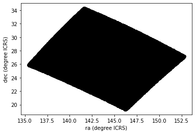
The arguments to plt.plot are x, y, and a string that specifies the style. In this case, the letters ko indicate that we want a black, round marker (k is for black because b is for blue).
The functions xlabel and ylabel put labels on the axes.
Looking at this plot, we can see that the region we selected, which is a rectangle in GD-1 coordinates, is a non-rectanglar region in ICRS coordinates.
However, this scatter plot has a problem. It is “overplotted”, which means that there are so many overlapping points, we can’t distinguish between high and low density areas.
To fix this, we can provide optional arguments to control the size and transparency of the points.
Exercise
In the call to plt.plot, use the keyword argument markersize to make the markers smaller.
Then add the keyword argument alpha to make the markers partly transparent.
Adjust these arguments until you think the figure shows the data most clearly.
Note: Once you have made these changes, you might notice that the figure shows stripes with lower density of stars. These stripes are caused by the way Gaia scans the sky, which you can read about here. The dataset we are using, Gaia Data Release 2, covers 22 months of observations; during this time, some parts of the sky were scanned more than others.
# Solution

# x = results['ra']
# y = results['dec']
# plt.plot(x, y, 'ko', markersize=0.1, alpha=0.1)

# plt.xlabel('ra (degree ICRS)')
# plt.ylabel('dec (degree ICRS)');
Transform back
Remember that we selected data from a rectangle of coordinates in the GD1Koposov10 frame, then transformed them to ICRS when we constructed the query.
The coordinates in results are in ICRS.
To plot them, we will transform them back to the GD1Koposov10 frame; that way, the axes of the figure are aligned with the orbit of GD-1, which is useful for two reasons:
By transforming the coordinates, we can identify stars that are likely to be in GD-1 by selecting stars near the centerline of the stream, where \(\phi_2\) is close to 0.
By transforming the proper motions, we can identify stars with non-zero proper motion along the \(\phi_1\) axis.
To do the transformation, we’ll put the results into a SkyCoord object. In a previous lesson we created a SkyCoord object like this:
from astropy.coordinates import SkyCoord

skycoord = SkyCoord(ra=results['ra'], dec=results['dec'])
Now we’re going to do something similar, but in addition to ra and dec, we’ll also include:
pmraandpmdec, which are proper motion in the ICRS frame, anddistanceandradial_velocity, which we explain below.
import astropy.units as u

distance = 8 * u.kpc
radial_velocity= 0 * u.km/u.s

skycoord = SkyCoord(ra=results['ra'],
                    dec=results['dec'],
                    pm_ra_cosdec=results['pmra'],
                    pm_dec=results['pmdec'],
                    distance=distance,
                    radial_velocity=radial_velocity)
For the first four arguments, we use columns from results.
For distance and radial_velocity we use constants, which we explain below.
The result is an Astropy SkyCoord object, which we can transform to the GD-1 frame.
from gala.coordinates import GD1Koposov10

gd1_frame = GD1Koposov10()
transformed = skycoord.transform_to(gd1_frame)
The result is another SkyCoord object, now in the GD1Koposov10 frame.
Reflex Correction
The next step is to correct the proper motion measurements for the effect of the motion of our solar system around the Galactic center.
When we created skycoord, we provided constant values for distance and radial_velocity rather than measurements from Gaia.
That might seem like a strange thing to do, but here’s the motivation:
Because the stars in GD-1 are so far away, the distance estimates we get from Gaia, which are based on parallax, are not very precise. So we replace them with our current best estimate of the mean distance to GD-1, about 8 kpc. See Koposov, Rix, and Hogg, 2010.
For the other stars in the table, this distance estimate will be inaccurate, so reflex correction will not be correct. But that should have only a small effect on our ability to identify stars with the proper motion we expect for GD-1.
The measurement of radial velocity has no effect on the correction for proper motion, but we have to provide a value to avoid errors in the reflex correction calculation. So we provide
0as an arbitrary place-keeper.
With this preparation, we can use reflex_correct from Gala (documentation here) to correct for the motion of the solar system.
from gala.coordinates import reflex_correct

skycoord_gd1 = reflex_correct(transformed)
The result is a SkyCoord object that contains
phi1andphi2, which represent the transformed coordinates in theGD1Koposov10frame.pm_phi1_cosphi2andpm_phi2, which represent the transformed and corrected proper motions.
We can select the coordinates and plot them like this:
x = skycoord_gd1.phi1
y = skycoord_gd1.phi2
plt.plot(x, y, 'ko', markersize=0.1, alpha=0.1)

plt.xlabel('phi1 (degree GD1)')
plt.ylabel('phi2 (degree GD1)');
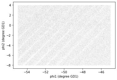
Remember that we started with a rectangle in the GD-1 frame. When transformed to the ICRS frame, it’s a non-rectangular region. Now, transformed back to the GD-1 frame, it’s a rectangle again.
Pandas DataFrame
At this point we have two objects containing different subsets of the data. results is the Astropy Table we downloaded from Gaia.
type(results)
astropy.table.table.Table
And skycoord_gd1 is a SkyCoord object that contains the transformed coordinates and proper motions.
type(skycoord_gd1)
astropy.coordinates.sky_coordinate.SkyCoord
On one hand, this division of labor makes sense because each object provides different capabilities. But working with multiple object types can be awkward.
It will be more convenient to choose one object and get all of the data into it. We’ll choose a Pandas DataFrame, for two reasons:
It provides capabilities that (almost) a superset of the other data structures, so it’s the all-in-one solution.
Pandas is a general-purpose tool that is useful in many domains, especially data science. If you are going to develop expertise in one tool, Pandas is a good choice.
However, compared to an Astropy Table, Pandas has one big drawback: it does not keep the metadata associated with the table, including the units for the columns.
It’s easy to convert a Table to a Pandas DataFrame.
import pandas as pd

results_df = results.to_pandas()
DataFrame provides shape, which shows the number of rows and columns.
results_df.shape
(140339, 6)
It also provides head, which displays the first few rows. head is useful for spot-checking large results as you go along.
results_df.head()
| source_id | ra | dec | pmra | pmdec | parallax | |
|---|---|---|---|---|---|---|
| 0 | 637987125186749568 | 142.483019 | 21.757716 | -2.516838 | 2.941813 | -0.257345 |
| 1 | 638285195917112960 | 142.254529 | 22.476168 | 2.662702 | -12.165984 | 0.422728 |
| 2 | 638073505568978688 | 142.645286 | 22.166932 | 18.306747 | -7.950660 | 0.103640 |
| 3 | 638086386175786752 | 142.577394 | 22.227920 | 0.987786 | -2.584105 | -0.857327 |
| 4 | 638049655615392384 | 142.589136 | 22.110783 | 0.244439 | -4.941079 | 0.099625 |
Python detail: shape is an attribute, so we display its value without calling it as a function; head is a function, so we need the parentheses.
Now we can extract the columns we want from skycoord_gd1 and add them as columns in the DataFrame. phi1 and phi2 contain the transformed coordinates.
results_df['phi1'] = skycoord_gd1.phi1
results_df['phi2'] = skycoord_gd1.phi2
results_df.shape
(140339, 8)
pm_phi1_cosphi2 and pm_phi2 contain the components of proper motion in the transformed frame.
results_df['pm_phi1'] = skycoord_gd1.pm_phi1_cosphi2
results_df['pm_phi2'] = skycoord_gd1.pm_phi2
results_df.shape
(140339, 10)
Detail: If you notice that SkyCoord has an attribute called proper_motion, you might wonder why we are not using it.
We could have: proper_motion contains the same data as pm_phi1_cosphi2 and pm_phi2, but in a different format.
Exploring data
One benefit of using Pandas is that it provides functions for exploring the data and checking for problems.
One of the most useful of these functions is describe, which computes summary statistics for each column.
results_df.describe()
| source_id | ra | dec | pmra | pmdec | parallax | phi1 | phi2 | pm_phi1 | pm_phi2 | |
|---|---|---|---|---|---|---|---|---|---|---|
| count | 1.403390e+05 | 140339.000000 | 140339.000000 | 140339.000000 | 140339.000000 | 140339.000000 | 140339.000000 | 140339.000000 | 140339.000000 | 140339.000000 |
| mean | 6.792399e+17 | 143.823122 | 26.780285 | -2.484404 | -6.100777 | 0.179492 | -50.091158 | -1.803301 | -0.868963 | 1.409208 |
| std | 3.792177e+16 | 3.697850 | 3.052592 | 5.913939 | 7.202047 | 0.759590 | 2.892344 | 3.444398 | 6.657714 | 6.518615 |
| min | 6.214900e+17 | 135.425699 | 19.286617 | -106.755260 | -138.065163 | -15.287602 | -54.999989 | -8.029159 | -115.275637 | -161.150142 |
| 25% | 6.443517e+17 | 140.967966 | 24.592490 | -5.038789 | -8.341561 | -0.035981 | -52.602952 | -4.750426 | -2.948723 | -1.107128 |
| 50% | 6.888060e+17 | 143.734409 | 26.746261 | -1.834943 | -4.689596 | 0.362708 | -50.147362 | -1.671502 | 0.585037 | 1.987149 |
| 75% | 6.976579e+17 | 146.607350 | 28.990500 | 0.452893 | -1.937809 | 0.657637 | -47.593279 | 1.160514 | 3.001768 | 4.628965 |
| max | 7.974418e+17 | 152.777393 | 34.285481 | 104.319923 | 20.981070 | 0.999957 | -44.999985 | 4.014609 | 39.802471 | 79.275199 |
Exercise
Review the summary statistics in this table.
Do the values make sense based on what you know about the context?
Do you see any values that seem problematic, or evidence of other data issues?
# Solution

# The most noticeable issue is that some of the
# parallax values are negative, which is non-physical.

# The reason is that parallax measurements are less accurate
# for stars that are far away.

# Fortunately, we don't use the parallax measurements in
# the analysis (one of the reasons we used constant distance
# for reflex correction).
Plot proper motion
Now we are ready to replicate one of the panels in Figure 1 of the Price-Whelan and Bonaca paper, the one that shows components of proper motion as a scatter plot:

In this figure, the shaded area identifies stars that are likely to be in GD-1 because:
Due to the nature of tidal streams, we expect the proper motion for stars in GD-1 to be along the axis of the stream; that is, we expect motion in the direction of
phi2to be near 0.In the direction of
phi1, we don’t have a prior expectation for proper motion, except that it should form a cluster at a non-zero value.
By plotting proper motion in the GD-1 frame, we hope to find this cluster. Then we will use the bounds of the cluster to select stars that are more likely to be in GD-1.
The following figure is a scatter plot of proper motion, in the GD-1 frame, for the stars in results_df.
x = results_df['pm_phi1']
y = results_df['pm_phi2']
plt.plot(x, y, 'ko', markersize=0.1, alpha=0.1)

plt.xlabel('Proper motion phi1 (mas/yr GD1 frame)')
plt.ylabel('Proper motion phi2 (mas/yr GD1 frame)');
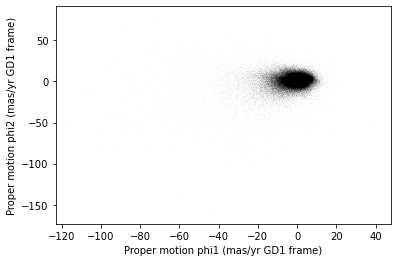
Most of the proper motions are near the origin, but there are a few extreme values.
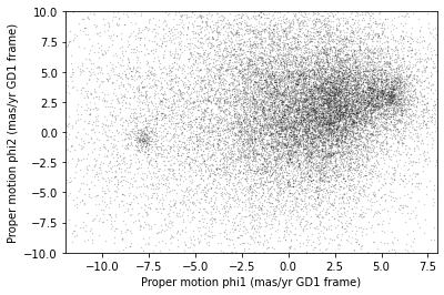
Following the example in the paper, we’ll use xlim and ylim to zoom in on the region near the origin.
x = results_df['pm_phi1']
y = results_df['pm_phi2']
plt.plot(x, y, 'ko', markersize=0.1, alpha=0.1)

plt.xlabel('Proper motion phi1 (mas/yr GD1 frame)')
plt.ylabel('Proper motion phi2 (mas/yr GD1 frame)')

plt.xlim(-12, 8)
plt.ylim(-10, 10);
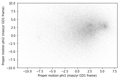
There is a hint of an overdense region near (-7.5, 0), but if you didn’t know where to look, you would miss it.
To see the cluster more clearly, we need a sample that contains a higher proportion of stars in GD-1. We’ll do that by selecting stars close to the centerline.
Selecting the centerline
As we can see in the following figure, many stars in GD-1 are less than 1 degree from the line phi2=0.

Stars near this line have the highest probability of being in GD-1.
To select them, we will use a “Boolean mask”. We’ll start by selecting the phi2 column from the DataFrame:
phi2 = results_df['phi2']
type(phi2)
pandas.core.series.Series
The result is a Series, which is the structure Pandas uses to represent columns.
We can use a comparison operator, >, to compare the values in a Series to a constant.
phi2_min = -1.0 * u.degree
phi2_max = 1.0 * u.degree

mask = (phi2 > phi2_min)
type(mask)
pandas.core.series.Series
The result is a Series of Boolean values, that is, True and False.
mask.head()
0    False
1    False
2    False
3    False
4    False
Name: phi2, dtype: bool
To select values that fall between phi2_min and phi2_max, we’ll use the & operator, which computes “logical AND”.
The result is true where elements from both Boolean Series are true.
mask = (phi2 > phi2_min) & (phi2 < phi2_max)
Python detail: Python’s logical operators (and, or, and not) don’t work with NumPy or Pandas. Both libraries use the bitwise operators (&, |, and ~) to do elementwise logical operations (explanation here).
Also, we need the parentheses around the conditions; otherwise the order of operations is incorrect.
The sum of a Boolean Series is the number of True values, so we can use sum to see how many stars are in the selected region.
mask.sum()
25084
A Boolean Series is sometimes called a “mask” because we can use it to mask out some of the rows in a DataFrame and select the rest, like this:
centerline_df = results_df[mask]
type(centerline_df)
pandas.core.frame.DataFrame
centerline_df is a DataFrame that contains only the rows from results_df that correspond to True values in mask.
So it contains the stars near the centerline of GD-1.
We can use len to see how many rows are in centerline_df:
len(centerline_df)
25084
And what fraction of the rows we’ve selected.
len(centerline_df) / len(results_df)
0.1787386257562046
There are about 25,000 stars in this region, about 18% of the total.
Plotting proper motion
Since we’ve plotted proper motion several times, let’s put that code in a function.
def plot_proper_motion(df):
    """Plot proper motion.

    df: DataFrame with `pm_phi1` and `pm_phi2`
    """
    x = df['pm_phi1']
    y = df['pm_phi2']
    plt.plot(x, y, 'ko', markersize=0.3, alpha=0.3)

    plt.xlabel('Proper motion phi1 (mas/yr GD1 frame)')
    plt.ylabel('Proper motion phi2 (mas/yr GD1 frame)')

    plt.xlim(-12, 8)
    plt.ylim(-10, 10)
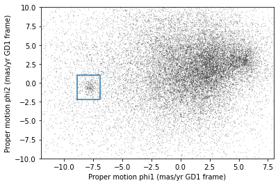
And we can call it like this:
plot_proper_motion(centerline_df)
Now we can see more clearly that there is a cluster near (-7.5, 0).
You might notice that our figure is less dense than the one in the paper. That’s because we started with a set of stars from a relatively small region. The figure in the paper is based on a region about 10 times bigger.
In the next lesson we’ll go back and select stars from a larger region. But first we’ll use the proper motion data to identify stars likely to be in GD-1.
Filtering based on proper motion
The next step is to select stars in the “overdense” region of proper motion, which are candidates to be in GD-1.
In the original paper, Price-Whelan and Bonaca used a polygon to cover this region, as shown in this figure.
We’ll use a simple rectangle for now, but in a later lesson we’ll see how to select a polygonal region as well.
Here are bounds on proper motion we chose by eye:
pm1_min = -8.9
pm1_max = -6.9
pm2_min = -2.2
pm2_max =  1.0
To draw these bounds, we’ll use make_rectangle to make two lists containing the coordinates of the corners of the rectangle.
def make_rectangle(x1, x2, y1, y2):
    """Return the corners of a rectangle."""
    xs = [x1, x1, x2, x2, x1]
    ys = [y1, y2, y2, y1, y1]
    return xs, ys
pm1_rect, pm2_rect = make_rectangle(
    pm1_min, pm1_max, pm2_min, pm2_max)
Here’s what the plot looks like with the bounds we chose.
plot_proper_motion(centerline_df)
plt.plot(pm1_rect, pm2_rect, '-');
Now that we’ve identified the bounds of the cluster in proper motion, we’ll use it to select rows from results_df.
We’ll use the following function, which uses Pandas operators to make a mask that selects rows where series falls between low and high.
def between(series, low, high):
    """Check whether values are between `low` and `high`."""
    return (series > low) & (series < high)
The following mask selects stars with proper motion in the region we chose.
pm1 = results_df['pm_phi1']
pm2 = results_df['pm_phi2']

pm_mask = (between(pm1, pm1_min, pm1_max) &
           between(pm2, pm2_min, pm2_max))
Again, the sum of a Boolean series is the number of True values.
pm_mask.sum()
1049
Now we can use this mask to select rows from results_df.
selected_df = results_df[pm_mask]
len(selected_df)
1049
These are the stars we think are likely to be in GD-1. Let’s see what they look like, plotting their coordinates (not their proper motion).
x = selected_df['phi1']
y = selected_df['phi2']
plt.plot(x, y, 'ko', markersize=1, alpha=1)

plt.xlabel('phi1 (degree GD1)')
plt.ylabel('phi2 (degree GD1)');
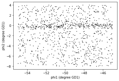
Now that’s starting to look like a tidal stream!
Saving the DataFrame
At this point we have run a successful query and cleaned up the results; this is a good time to save the data.
To save a Pandas DataFrame, one option is to convert it to an Astropy Table, like this:
selected_table = Table.from_pandas(selected_df)
type(selected_table)
astropy.table.table.Table
Then we could write the Table to a FITS file, as we did in the previous lesson.
But Pandas provides functions to write DataFrames in other formats; to see what they are find the functions here that begin with to_.
One of the best options is HDF5, which is Version 5 of Hierarchical Data Format.
HDF5 is a binary format, so files are small and fast to read and write (like FITS, but unlike XML).
An HDF5 file is similar to an SQL database in the sense that it can contain more than one table, although in HDF5 vocabulary, a table is called a Dataset. (Multi-extension FITS files can also contain more than one table.)
And HDF5 stores the metadata associated with the table, including column names, row labels, and data types (like FITS).
Finally, HDF5 is a cross-language standard, so if you write an HDF5 file with Pandas, you can read it back with many other software tools (more than FITS).
We can write a Pandas DataFrame to an HDF5 file like this:
filename = 'gd1_data.hdf'

selected_df.to_hdf(filename, 'selected_df', mode='w')
Because an HDF5 file can contain more than one Dataset, we have to provide a name, or “key”, that identifies the Dataset in the file.
We could use any string as the key, but it will be convenient to give the Dataset in the file the same name as the DataFrame.
The argument mode='w' means that if the file already exists, we should overwrite it.
Exercise
We’re going to need centerline_df later as well. Write a line of code to add it as a second Dataset in the HDF5 file.
Hint: Since the file already exists, you should not use mode='w'.
# Solution

centerline_df.to_hdf(filename, 'centerline_df')
We can use getsize to confirm that the file exists and check the size:
from os.path import getsize

MB = 1024 * 1024
getsize(filename) / MB
2.2084197998046875
If you forget what the names of the Datasets in the file are, you can read them back like this:
with pd.HDFStore(filename) as hdf:
    print(hdf.keys())
['/centerline_df', '/selected_df']
Python note: We use a with statement here to open the file before the print statement and (automatically) close it after. Read more about context managers.
The keys are the names of the Datasets. Notice that they start with /, which indicates that they are at the top level of the Dataset hierarchy, and not in a named “group”.
In future lessons we will add a few more Datasets to this file, but not so many that we need to organize them into groups.
Summary
In this lesson, we re-loaded the Gaia data we saved from a previous query.
We transformed the coordinates and proper motion from ICRS to a frame aligned with the orbit of GD-1, and stored the results in a Pandas DataFrame.
Then we replicated the selection process from the Price-Whelan and Bonaca paper:
We selected stars near the centerline of GD-1 and made a scatter plot of their proper motion.
We identified a region of proper motion that contains stars likely to be in GD-1.
We used a Boolean
Seriesas a mask to select stars whose proper motion is in that region.
So far, we have used data from a relatively small region of the sky. In the next lesson, we’ll write a query that selects stars based on proper motion, which will allow us to explore a larger region.
Best practices
When you make a scatter plot, adjust the size of the markers and their transparency so the figure is not overplotted; otherwise it can misrepresent the data badly.
For simple scatter plots in Matplotlib,
plotis faster thanscatter.An Astropy
Tableand a PandasDataFrameare similar in many ways and they provide many of the same functions. They have pros and cons, but for many projects, either one would be a reasonable choice.To store data from a Pandas
DataFrame, a good option is an HDF file, which can contain multiple Datasets.