11. Second-Order Systems

Run this chapter online (or with solutions)

So far we’ve seen first-order differential equations and systems of first-order ODEs. In this chapter, we’ll introduce second-order systems, which are particularly useful for modeling Newtonian motion.

Newtonian Motion

Newton’s second law of motion is often written like this:

\[ \begin{align}\begin{aligned}F = m a$$ where $F$ is the net force acting on an object, $m$ is the mass of the object, and $a$ is the acceleration of the object.\\This equation suggests that if you know $m$ and $a$, you can compute the force. And that’s true, but in most physical simulations it’s the other way around: based on a physical model, you know $F$ and $m$, and you compute $a$.\\So if we know acceleration as a function of time, how do we find the position of the object, $r$? Well, we know that acceleration is the second derivative of position, so we can write the differential equation\\$$\frac{d^2r}{dt^2} = a$$ where ${d^2r}/{dt^2}$ is the second time derivative of $r$.\\Because this equation includes a second derivative, it’s a second-order ODE. We can’t solve the equation using `ode45` in this form, but by introducing a new variable, *v*, for velocity, we can rewrite it as a system of first-order ODEs:\\\begin{split}$$\begin{aligned} \frac{dr}{dt} &= v \\ \frac{dv}{dt} &= a \end{aligned}\end{split}\end{aligned}\end{align} \]

The first equation says that the first derivative of \(r\) is \(v\); the second equation says that the first derivative of \(v\) is \(a\).

Free Fall

As an example of Newtonian motion, let’s go back to the question from Exercise 1.1:

If you drop a penny from the top of the Empire State Building, how long does it take to reach the sidewalk, and how fast is it going when it gets there?

We’ll start with no air resistance; then we’ll add air resistance to the model and see what effect it has.

Near the surface of the earth, acceleration due to gravity is -9.8 m/s², where the minus sign indicates that gravity pulls down. If the object falls straight down, we can describe its position with a scalar value \(y\), representing altitude.

Listing 11.1 contains a rate function we can use with ode45 to solve this problem:

Listing 11.1: A rate function for the falling penny problem

function res = rate_func(t, X)
    % unpack position and velocity
    y = X(1);
    v = X(2);

    % compute the derivatives
    dydt = v;
    dvdt = -9.8;

    % pack the derivatives into a column vector
    res = [dydt; dvdt];
end

The rate function in Listing 11.1 takes t and X as input variables, where the elements of X are understood to be the position and velocity of the penny.

It returns a column vector that contains dydt and dvdt, which are velocity and acceleration, respectively. Since velocity is the second element of X, we can simply assign this value to dydt. And since the derivative of velocity is acceleration, we can assign the acceleration due to gravity to dvdt.

As always, we should test the rate function before we call ode45. Here’s the top-level function we can use to test it:

function penny()
   t = 0;
   X = [381, 0];
   rate_func(t, X)
end

The initial condition of X is the initial position, which is the height of the Empire State Building, about 381 m, and the initial velocity, which is 0 m/s.

The result from rate_func is

penny

ans =

        0
  -9.8000

which is what we expect.

Now we can run ode45 with this rate function:

X = [381, 0];    % the initial condition, as in penny
tspan = [0, 10]
[T, M] = ode45(@rate_func, tspan, X)

tspan =

    0   10
T =

         0
    0.0170
    0.0341
    0.0511
    0.0681
    0.0937
    0.1192
    0.1448
    0.1703
    0.2086
    0.2470
    0.2853
    0.3236
    0.3811
    0.4386
    0.4961
    0.5535
    0.6398
    0.7260
    0.8122
    0.8985
    1.0278
    1.1571
    1.2865
    1.4158
    1.6098
    1.8038
    1.9978
    2.1918
    2.4418
    2.6918
    2.9418
    3.1918
    3.4418
    3.6918
    3.9418
    4.1918
    4.4418
    4.6918
    4.9418
    5.1918
    5.4418
    5.6918
    5.9418
    6.1918
    6.4418
    6.6918
    6.9418
    7.1918
    7.4418
    7.6918
    7.9418
    8.1918
    8.4418
    8.6918
    8.9418
    9.1918
    9.3939
    9.5959
    9.7980
   10.0000

M =

   381.0000          0
   380.9986    -0.1669
   380.9943    -0.3338
   380.9872    -0.5007
   380.9773    -0.6677
   380.9570    -0.9180
   380.9303    -1.1684
   380.8973    -1.4188
   380.8579    -1.6692
   380.7867    -2.0447
   380.7011    -2.4203
   380.6012    -2.7959
   380.4868    -3.1714
   380.2883    -3.7348
   380.0575    -4.2981
   379.7942    -4.8614
   379.4986    -5.4248
   378.9944    -6.2698
   378.4173    -7.1148
   377.7674    -7.9598
   377.0446    -8.8048
   375.8238   -10.0724
   374.4391   -11.3399
   372.8905   -12.6074
   371.1779   -13.8749
   368.3016   -15.7762
   365.0564   -17.6775
   361.4424   -19.5788
   357.4595   -21.4801
   351.7832   -23.9301
   345.4945   -26.3801
   338.5932   -28.8301
   331.0794   -31.2801
   322.9532   -33.7301
   314.2144   -36.1801
   304.8631   -38.6301
   294.8994   -41.0801
   284.3231   -43.5301
   273.1343   -45.9801
   261.3331   -48.4301
   248.9193   -50.8801
   235.8930   -53.3301
   222.2542   -55.7801
   208.0030   -58.2301
   193.1392   -60.6801
   177.6629   -63.1301
   161.5742   -65.5801
   144.8729   -68.0301
   127.5591   -70.4801
   109.6329   -72.9301
    91.0941   -75.3801
    71.9428   -77.8301
    52.1791   -80.2801
    31.8028   -82.7301
    10.8140   -85.1801
   -10.7872   -87.6301
   -33.0010   -90.0801
   -51.4007   -92.0601
   -70.2004   -94.0400
   -89.4002   -96.0200
  -109.0000   -98.0000

As always, the first argument is the function handle, the second is the time span (10 seconds), and the third is the initial condition.

The result is a vector, T, that contains the time values, and a matrix, M, that contains two columns, one for altitude and one for velocity.

We can extract the first column and plot it, like this:

Y = M(:, 1)
plot(T, Y)

Y =

   381.000
   380.999
   380.994
   380.987
   380.977
   380.957
   380.930
   380.897
   380.858
   380.787
   380.701
   380.601
   380.487
   380.288
   380.057
   379.794
   379.499
   378.994
   378.417
   377.767
   377.045
   375.824
   374.439
   372.890
   371.178
   368.302
   365.056
   361.442
   357.460
   351.783
   345.494
   338.593
   331.079
   322.953
   314.214
   304.863
   294.899
   284.323
   273.134
   261.333
   248.919
   235.893
   222.254
   208.003
   193.139
   177.663
   161.574
   144.873
   127.559
   109.633
    91.094
    71.943
    52.179
    31.803
    10.814
   -10.787
   -33.001
   -51.401
   -70.200
   -89.400
  -109.000

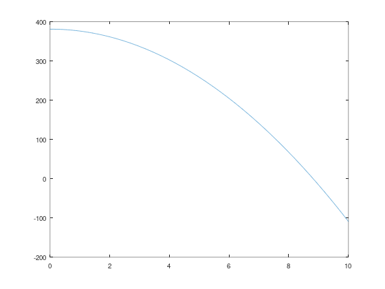
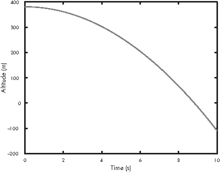
Figure 11.1: Altitude versus time for an object in free fall

Figure 11.1 shows the result. Altitude drops slowly at first and picks up speed. Between 8 and 9 seconds, the altitude reaches 0, which means the penny hits the sidewalk. But ode45 doesn’t know where the ground is, so the penny keeps going through 0 into negative altitude. We’ll solve that problem in the next section.

ODE Events

Normally when you call ode45 you specify a start time and an end time. But sometimes you don’t know ahead of time when the simulation should end. To solve this problem we can define an event, something of interest that happens during a simulation, like the penny reaching the ground.

Here are the steps:

1. First we define an event function that allows ode45 to figure out when an event occurs. Here’s an event function for the penny example:

function [value, isterminal, direction] = event_func(t,X)
    value = X(1);
    isterminal = 1;
    direction = -1;
end

The event function takes the same input variables as the rate function and returns three output variables: value determines when an event can occur, direction determines whether it does, and isterminal determines what happens. More specifically, an event can occur when value passes through 0. If direction is positive, the event only occurs if value is increasing. If direction is negative, the event only occurs if value is decreasing. If direction is 0, the event always occurs. If isterminal is 1, the event causes the simulation to end; if it is 0, the simulation continues.

This event function uses the altitude of the penny as value so an event can occur when altitude passes through 0. Because direction is negative, an event occurs only when altitude is decreasing, and because isterminal is 1, the simulation ends if an event occurs.

2. Next, we use odeset to create an object called options:

options = odeset('Events', @event_func);

The name of the option is Events and the value is the handle of the event function.

3. Finally, we pass options as a fourth argument to ode45:

[T, M] = ode45(@rate_func, tspan, X, options);

When ode45 runs, it invokes event_func after each time step. If the event function indicates that a terminal event occurred, ode45 stops the simulation.

Let’s look at the results from the penny example:

T(end)
M(end, :)

ans = 8.8179
ans =

  -3.5127e-13  -8.6415e+01

The last value of T is about 8.8, which is the number of seconds the penny takes to reach the sidewalk.

The last row of M indicates that the final altitude is 0, which is what we wanted, and the final velocity is about -86 m/s.

Air Resistance

To make this simulation more realistic, we can add air resistance. For large objects moving quickly through air, the force due to air resistance, called drag, is proportional to velocity squared. For an object falling down, drag is directed up, so if velocity is negative, drag force is positive.

Here’s how we can compute the force of drag as a function of velocity in one dimension:

$\(f_\mathrm{d} = -\mathrm{sign}(v) b v^2\)\( where \)v\( is velocity and \)b$ is a drag constant that depends on the density of air, the cross-sectional area of the object, and the shape of the object.

The sign or signum function returns the value \(1\) for positive values of \(v\) and \(-1\) for negative values. So \(f_\mathrm{d}\) is always in the opposite direction of \(v\).

To convert from force to acceleration we have to know mass, but that’s easy to find: the mass of a penny is about 2.5 g. It’s not as easy to find the drag constant, but based on reports that the terminal velocity of a penny is about 18 m/s, I’ve estimated that it’s about 75e-6 kg/m.

Listing 11.2 defines a function that takes t and X as input variables and returns the total acceleration of the penny due to gravity and drag:

Listing 11.2: Calculating acceleration of a penny with drag

function res = acceleration(t, X)
    b = 75e-6;                 % drag constant in kg/m
    v = X(2);                  % velocity in m/s
    f_d = -sign(v) * b * v^2;  % drag force in N

    m = 2.5e-3;               % mass in kg
    a_d = f_d / m;            % drag acceleration in m/s^2

    a_g = -9.8;               % acceleration of gravity in m/s^2
    res = a_g + a_d;          % total acceleration
end

First, we compute force due to drag. Then we compute acceleration due to drag. Lastly, we compute total acceleration due to drag and gravity.

Be careful when you’re working with forces and accelerations; make sure you only add forces to forces or accelerations to accelerations. In my code, I use comments to remind myself what units the values have. That helps me avoid errors like adding forces to accelerations.

To use this function, we make a small change in rate_func:

function res = rate_func(t, X)
    y = X(1);
    v = X(2);

    dydt = v;
    dvdt = acceleration(t, X);   % this line has changed

    res = [dydt; dvdt];
end

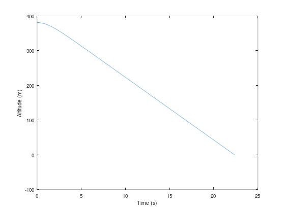
% Run the simulation again with drag (Figure 11.2). The penny takes longer
% to reach the ground, so the time span is longer.
tspan = [0, 30];
[T, M] = ode45(@rate_func, tspan, X, options);
plot(T, M(:, 1))
xlabel('Time (s)')
ylabel('Altitude (m)')
T(end)
M(end, :)

ans = 22.358
ans =

  -2.4081e-13  -1.8074e+01

In the previous version, dvdt is always -9.8, the acceleration due to gravity. In this version, we call acceleration to compute the total acceleration due to gravity and drag.

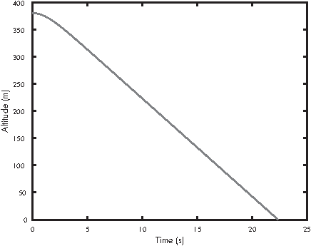
Figure 11.2: Altitude versus time for a penny in free fall with air resistance

Everything else is the same. Figure 11.2 shows the result.

Air resistance makes a big difference! Velocity increases until acceleration due to drag equals acceleration due to gravity; after that, velocity is constant and position decreases linearly (and much more slowly than it would in a vacuum).

With air resistance, the time until the penny hits the sidewalk is 22.4 s, substantially longer than before (8.8 s).

And the final velocity is 18.1 m/s, substantially slower than before (86 m/s).

Chapter Review

In this chapter, we used Newton’s laws of motion to write a differential equation that describes the motion of a falling penny.

We rewrote that equation as a system of first-order differential equations so we could use ode45 to solve it. Then we ran simulations of a falling penny with and without air resistance, also known as drag.

We defined an event as something of interest that happens during a simulation, like a collision between moving objects, and we wrote an event function, which allows ode45 to figure out when an event occurs.

In the next chapter, we extend Newtonian motion to two dimensions and model the flight of a baseball.

Exercises

Before you go on, you might want to work on the following exercise.

Exercise 11.1.

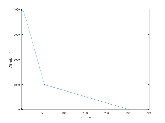
In this exercise we’ll model the descent of a skydiver, taking into account the change in drag when the parachute opens.

1. Modify the penny code from this chapter to simulate the descent of a 75 kg skydiver from an initial altitude of 4000 m. The drag constant for a skydiver without a parachute is about 0.2 kg/m. What would the velocity of the skydiver be on impact?

2. After opening their parachute, the velocity of the skydiver slows to about 5 m/s. Use your simulation to find the drag constant that yields a terminal velocity of 5 m/s.

3. Increase the mass of the skydiver, and confirm that terminal velocity increases. This phenomenon is the source of the intuition that heavy objects fall faster; in air, they do!

4. Now suppose the skydiver free falls until they get to an altitude of 1000 m before opening the parachute. How long would it take them to reach the ground?

5. What is the lowest altitude where the skydiver can open the parachute and still land at less than 6 m/s (assuming that the parachute opens and deploys instantly)?

Exercise 11.2.

Here’s a question from the website Ask an Astronomer (see https://greenteapress.com/matlab/astro):

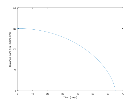
If the Earth suddenly stopped orbiting the Sun, I know eventually it would be pulled in by the Sun’s gravity and hit it. How long would it take the Earth to hit the Sun? I imagine it would go slowly at first and then pick up speed.

Use ode45 to answer this question. Here are some suggestions about how to proceed:

1. Look up the Law of Universal Gravitation and any constants you need. I suggest you work entirely in SI units: meters, kilograms, and newtons.

2. When the distance between the Earth and the Sun gets small, this system behaves badly, so you should use an event function to stop when the surface of the Earth reaches the surface of the Sun.

3. Express your answer in days, and plot the results as millions of kilometers versus days.

Show solution

Hide solution

% Solution

% Simulate the descent of a skydiver who opens the parachute at altitude
% h_open (default 1000 m).  The lowest altitude where they still land at
% less than 6 m/s is about 8 m (the last part of the exercise).

function skydiver(h_open)
    if nargin < 1
        h_open = 1000;        % altitude where the parachute opens, in m
    end
    t = 0;
    X = [4000, 0];
    rate_func(t, X, h_open)

    tspan = [0, 1000];
    options = odeset('Events', @event_func);
    [T, M] = ode45(@(t, X) rate_func(t, X, h_open), tspan, X, options);

    Y = M(:, 1);
    V = M(:, 2);

    plot(T, Y)
    xlabel('Time (s)')
    ylabel('Altitude (m)')

    T(end)
    M(end, :)
end

function res = rate_func(t, X, h_open)
    % unpack position and velocity
    y = X(1);
    v = X(2);

    % compute the derivatives
    dydt = v;
    dvdt = acceleration(t, X, h_open);

    % pack the derivatives into a column vector
    res = [dydt; dvdt];
end

function res = acceleration(t, X, h_open)
    b_free = 0.2;             % drag constant in kg/m
    b_parachute = 29;

    y = X(1);
    if y < h_open
        b = b_parachute;
    else
        b = b_free;
    end

    v = X(2);                 % velocity in m/s
    f_d = -sign(v) * b * v^2; % drag force in N

    m = 75;                   % mass in kg
    a_d = f_d / m;            % drag acceleration in m/s^2

    a_g = -9.8;               % acceleration due to gravity in m/s^2
    res = a_g + a_d;          % total acceleration
end

function [value, isterminal, direction] = event_func(t,X)
    value = X(1);
    isterminal = 1;
    direction = -1;
end

Show solution

Hide solution

% Solution

skydiver

ans =

        0

  -9.8000

ans = 251.30
ans =

   5.9586e-13  -5.0348e+00

Show solution

Hide solution

% Solution

% Simulate the Earth falling into the Sun.

function earth()
    y0 = 150e9;           % meters
    t_end = 1e7;          % seconds
    
    t = 0;
    X = [y0, 0];
    rate_func(t, X)
   
    tspan = [0, t_end];
    options = odeset('Events', @event_func);
    [T, M] = ode45(@rate_func, tspan, X, options);
    
    % convert time to days
    % convert distance to millions of km
    T = T / 60 / 60 / 24;
    Y = M(:, 1) / 1e9;
    
    plot(T, Y)
    xlabel('Time (days)')
    ylabel('Distance from sun (million km)')
    
    T(end)
    M(end, :)
end

function res = rate_func(t, X)
    % unpack position and velocity
    y = X(1);      
    v = X(2);      
    
    % compute the derivatives
    dydt = v;
    dvdt = acceleration(t, X);

    % pack the derivatives into a column vector
    res = [dydt; dvdt];
end

function res = acceleration(t, X)
    G=6.674e-11;          % N / kg^2 * m^2,
    m_sun = 1.989e30;     %  kg,
    m_earth = 5.972e24;   % kg,

    y = X(1);
    f_g = -G * m_earth * m_sun / y^2;
    a_g = f_g / m_earth;
    res = a_g;
end

function [value, isterminal, direction] = event_func(t, X)
    r_earth = 6.371e6;           % meters
    r_sun = 695.508e6;           % meters
    y_final = r_sun + r_earth;
    y = X(1);
    
    value = y - y_final;
    isterminal = 1;
    direction = -1;
end

Show solution

Hide solution

% Solution

earth

ans =

            0

  -5.8998e-03

ans = 64.813

ans =

   7.0188e+08  -6.1475e+05