10. Systems of ODEs

Run this chapter online (or with solutions)

In the previous chapter we used Euler’s method and ode45 to solve a single first-order differential equation. In this chapter, we’ll move on to systems of ODEs and implement a model of a predator-prey system. But first, we have to learn more about matrices.

Matrices

A matrix is a two-dimensional version of a vector. Like a vector, it contains elements that are identified by indices. The difference is that the elements are arranged in rows and columns, so it takes two indices to identify an element.

Creating a Matrix

A common way to create a matrix is the zeros function, which returns a matrix with the given size filled with zeros. This example creates a matrix with two rows and three columns.

M = zeros(2, 3)

M =

   0   0   0
   0   0   0

If you don’t know the size of a matrix, you can display it by using whos:

whos M

Variables visible from the current scope:

variables in scope: top scope

  Attr   Name        Size                     Bytes  Class
  ====   ====        ====                     =====  ===== 
         M           2x3                         48  double

Total is 6 elements using 48 bytes

or the size function, which returns a vector:

V = size(M)

V =

   2   3

The first element is the number of rows; the second is the number of columns.

To read an element of a matrix, you specify the row and column numbers:

M(1,2)
M(2,3)

ans = 0
ans = 0

When you’re working with matrices, it takes some effort to remember which index comes first, row or column. I find it useful to repeat “row, column” to myself, like a mantra. You might also find it helpful to remember “down, across” or the abbreviation RC as in “radio control” or RC Cola.

Another way to create a matrix is to enclose the elements in brackets, with semicolons between rows:

D = [1,2,3 ; 4,5,6]
size(D)

D =

   1   2   3
   4   5   6
ans =

   2   3

Row and Column Vectors

Although it’s useful to think in terms of numbers, vectors, and matrices, from MATLAB’s point of view everything is a matrix. A number is just a matrix that happens to have one row and one column:

x = 5;
size(x)

ans =

   1   1

And a vector is a matrix with only one row:

R = 1:5;
size(R)

ans =

   1   5

Well, some vectors have only one row, anyway. Actually, there are two kinds of vectors. The ones we’ve seen so far are called row vectors, because the elements are arranged in a row; the other kind are column vectors, where the elements are in a single column.

One way to create a column vector is to create a matrix with only one element per row:

C = [1;2;3]
size(C)

C =

   1
   2
   3
ans =

   3   1

The difference between row and column vectors is important in linear algebra, but for most basic vector operations, it doesn’t matter. For example, when you index the elements of a vector, you don’t have to know what kind it is:

R(2)
C(2)

ans = 2
ans = 2

The Transpose Operator

The transpose operator, which looks remarkably like an apostrophe, computes the transpose of a matrix, which is a new matrix that has all of the elements of the original, but with each row transformed into a column (or you can think of it the other way around).

In this example D has two rows:

D = [1,2,3 ; 4,5,6]

D =

   1   2   3
   4   5   6

so its transpose has two columns:

Dt = D'

Dt =

   1   4
   2   5
   3   6

Exercise 10.1. What effect does the transpose operator have on row vectors, column vectors, and numbers?

Solving Systems of ODEs

Now that we’ve seen the basics of matrices, let’s see how we can use them to solve systems of differential equations.

Lotka-Volterra

The Lotka-Volterra model describes the interactions between two species in an ecosystem, a predator and its prey. As an example, we’ll consider foxes and rabbits.

The model is governed by the following system of differential equations:

\[\begin{split}\begin{aligned} \frac{dx}{dt} &= a x - b x y \\ \frac{dy}{dt} &= -c y + d x y \end{aligned}\end{split}\]

where \(x\) and \(y\) are the populations of rabbits and foxes, and \(a\), \(b\), \(c\), and \(d\) are parameters that quantify the interactions between the two species (see https://greenteapress.com/matlab/lotka).

At first glance, you might think you could solve these equations by calling ode45 once to solve for \(x\) and once to solve for \(y\). The problem is that each equation involves both variables, which is what makes this a system of equations and not just a list of unrelated equations. To solve a system, you have to solve the equations simultaneously.

Fortunately, ode45 can handle systems of equations. The difference is that the initial condition is a vector that contains the initial values \(x(0)\) and \(y(0)\), and the output is a matrix that contains one column for \(x\) and one for \(y\).

Listing 10.1 shows the rate function with the parameters \(a = 0.1\), \(b = 0.01\), \(c = 0.1\), and \(d = 0.002\):

Listing 10.1: A rate function for Lotka-Volterra

function res = rate_func(t, V)
    % unpack the elements of V
    x = V(1);
    y = V(2);

    % set the parameters
    a = 0.1;
    b = 0.01;
    c = 0.1;
    d = 0.002;

    % compute the derivatives
    dxdt = a*x - b*x*y;
    dydt = -c*y + d*x*y;

    % pack the derivatives into a vector
    res = [dxdt; dydt];
end

The first input variable, t, is time. Even though the time variable is not used in this rate function, it has to be there in order for this function to work with ode45. The second input variable, V, is a vector with two elements, \(x(t)\) and \(y(t)\). The body of the function includes four sections, each explained by a comment.

The first section unpacks the vector by copying the elements into variables. This isn’t necessary, but giving names to these values will help you to remember what’s what. It also makes the third section, where we compute the derivatives, resemble the mathematical equations we were given, which helps prevent errors.

The second section sets the parameters that describe the reproductive rates of rabbits and foxes, and the characteristics of their interactions. If we were studying a real system, these values would come from observations of real animals, but for this example I chose values that yield interesting results.

The third section computes the derivatives of \(x\) and \(y\), using the equations we were given.

The last section packs the computed derivatives back into a vector. When ode45 calls this function, it provides a vector as input and expects to get a vector as output.

Sharp-eyed readers will notice something different about this line:

res = [dxdt; dydt];

The semicolon between the elements of the vector is not an error. It is necessary in this case because ode45 requires the result of this function to be a column vector.

As always, it’s a good idea to test your rate function before you call ode45. Create a file named lotka.m with the following top-level function:

function res = lotka()
    t = 0;
    V_init = [80, 20];
    rate_func(t, V_init)
end

lotka

ans =

  -8.0000
   1.2000

V_init is a vector that represents the initial condition, 80 rabbits and 20 foxes. The result from rate_func is

which means that with these initial conditions, we expect the rabbit population to decline initially at a rate of 8 per week and the fox population to increase by 1.2 per week.

Now we can run ode45 like this:

V_init = [80, 20];    % the initial condition, as in lotka
tspan = [0, 200]
[T, M] = ode45(@rate_func, tspan, V_init)

tspan =

     0   200
T =

          0
     0.0170
     0.0341
     0.0511
     0.0681
     0.0937
     0.1192
     0.1448
     0.1703
     0.2086
     0.2470
     0.2853
     0.3236
     0.3811
     0.4386
     0.4961
     0.5535
     0.6398
     0.7260
     0.8122
     0.8985
     1.0278
     1.1571
     1.2865
     1.4158
     1.6098
     1.8038
     1.9978
     2.1918
     2.4829
     2.7739
     3.0649
     3.3559
     3.7924
     4.2289
     4.6655
     5.1020
     5.7568
     6.4115
     7.0663
     7.7211
     8.7033
     9.6854
    10.6676
    11.6498
    13.1230
    14.5963
    16.0695
    17.5428
    19.2904
    21.0379
    22.7855
    24.5331
    26.8107
    29.0882
    31.3658
    33.6433
    37.0597
    40.4760
    43.8923
    47.3087
    49.9493
    52.5900
    55.2306
    57.8713
    59.5048
    61.1383
    62.7718
    64.4053
    66.2290
    68.0527
    69.8764
    71.7001
    73.5292
    75.3583
    77.1874
    79.0165
    80.9966
    82.9768
    84.9569
    86.9371
    88.7553
    90.5735
    92.3918
    94.2100
    96.8227
    99.4354
   102.0480
   104.6607
   108.3429
   112.0251
   115.7073
   119.3895
   122.8389
   126.2883
   129.7377
   133.1871
   134.8564
   136.5258
   138.1951
   139.8645
   141.4510
   143.0374
   144.6239
   146.2104
   148.2202
   150.2300
   152.2398
   154.2495
   156.0554
   157.8614
   159.6673
   161.4732
   164.0758
   166.6784
   169.2810
   171.8836
   175.5547
   179.2257
   182.8968
   186.5679
   189.9259
   193.2839
   196.6420
   200.0000

M =

    80.0000    20.0000
    79.8637    20.0204
    79.7274    20.0407
    79.5910    20.0610
    79.4546    20.0812
    79.2499    20.1113
    79.0452    20.1413
    78.8403    20.1711
    78.6354    20.2007
    78.3280    20.2449
    78.0204    20.2887
    77.7127    20.3320
    77.4050    20.3750
    76.9433    20.4388
    76.4816    20.5016
    76.0199    20.5636
    75.5584    20.6247
    74.8664    20.7145
    74.1751    20.8023
    73.4847    20.8880
    72.7954    20.9715
    71.7640    21.0927
    70.7364    21.2090
    69.7132    21.3202
    68.6952    21.4264
    67.1792    21.5760
    65.6784    21.7140
    64.1946    21.8402
    62.7297    21.9546
    60.5714    22.1039
    58.4642    22.2266
    56.4122    22.3230
    54.4191    22.3934
    51.5457    22.4515
    48.8175    22.4549
    46.2383    22.4062
    43.8094    22.3088
    40.4456    22.0792
    37.4072    21.7606
    34.6780    21.3658
    32.2384    20.9073
    29.0730    20.1258
    26.4310    19.2636
    24.2391    18.3514
    22.4324    17.4141
    20.3227    16.0032
    18.7936    14.6281
    17.7232    13.3211
    17.0275    12.1001
    16.6079    10.7740
    16.5595     9.5852
    16.8379     8.5311
    17.4188     7.6047
    18.6185     6.5728
    20.3335     5.7184
    22.6035     5.0200
    25.4880     4.4589
    31.1351     3.8430
    38.7144     3.4624
    48.5788     3.3084
    60.9764     3.4135
    72.2595     3.7290
    84.6967     4.3343
    97.1755     5.3770
   107.5034     7.0934
   111.4514     8.6127
   112.2363    10.5564
   109.0769    12.9008
   101.8526    15.4886
    89.7488    18.3224
    75.4102    20.6440
    61.0112    22.1009
    48.4595    22.5135
    38.6905    21.9709
    31.4014    20.7842
    26.2149    19.2099
    22.5799    17.4724
    19.8510    15.5835
    18.0981    13.7770
    17.0498    12.1185
    16.5702    10.6299
    16.5669     9.4122
    16.9129     8.3390
    17.5849     7.4018
    18.5756     6.5901
    20.5738     5.6201
    23.3108     4.8520
    26.8869     4.2577
    31.4309     3.8162
    39.7181     3.4359
    50.7995     3.3113
    64.9258     3.4894
    81.6150     4.1345
    98.7771     5.3352
   110.5002     7.9488
   109.6462    12.3258
    93.0348    17.6533
    80.3282    19.9422
    66.9819    21.5923
    54.4040    22.4474
    43.8772    22.4306
    36.2113    21.7199
    30.3251    20.5872
    25.9175    19.1993
    22.6755    17.6900
    19.8212    15.7520
    17.9937    13.8964
    16.8974    12.1947
    16.3908    10.6696
    16.3763     9.4489
    16.7054     8.3723
    17.3547     7.4315
    18.3164     6.6159
    20.2673     5.6373
    22.9447     4.8611
    26.4467     4.2590
    30.9001     3.8093
    39.0425     3.4150
    49.9484     3.2731
    63.9031     3.4257
    80.5245     4.0256
    97.2893     5.1343
   109.8505     7.4939
   111.6483    11.4931
    98.2226    16.6698

The first argument is the function handle for the rate function. The second argument is the time span, from 0 to 200 weeks. The third argument is the initial condition.

Output Matrices

The ode45 function returns two values: T, a vector, and M, a matrix.

size(T)
size(M)

ans =

   125     1
ans =

   125     2

T has 101 rows and 1 column, so it is a column vector with one row for each time step.

M has 101 rows, one for each time step, and 2 columns, one for each variable, \(x\) and \(y\).

This structure—one column per variable—is a common way to use matrices. And plot understands this structure, so if you do the following:

plot(T, M)

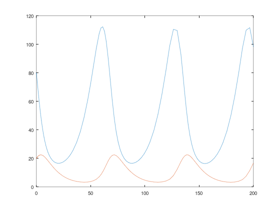
MATLAB understands that it should plot each column from M versus T.

You can copy the columns of M into other variables like this:

R = M(:, 1);
F = M(:, 2);

In this context, the colon represents the range from 1 to end, so M(:, 1) means “all the rows, column 1” and M(:, 2) means “all the rows, column 2.”

size(R)
size(F)

ans =

   125     1
ans =

   125     1

So R and F are column vectors.

Now we can plot these vectors separately, which makes it easier to give them different style strings:

hold on
plot(T, R, '-')
plot(T, F, '--')

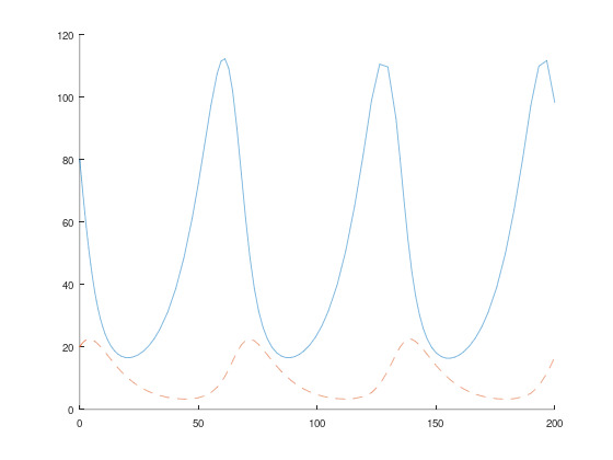
Figure 10.1 shows the results. The x-axis is time in weeks; the y-axis is population. The top curve shows the population of rabbits; the bottom curve shows foxes.

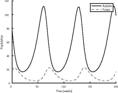
Figure 10.1: Solution for the Lotka-Volterra model

Initially, there are too many foxes, so the rabbit population declines. Then there are not enough rabbits, and the fox population declines. That allows the rabbit population to recover, and the pattern repeats.

This cycle of “boom and bust” is typical of the Lotka-Volterra model.

Phase Plot

Instead of plotting the two populations over time, it is sometimes useful to plot them against each other:

plot(R, F)

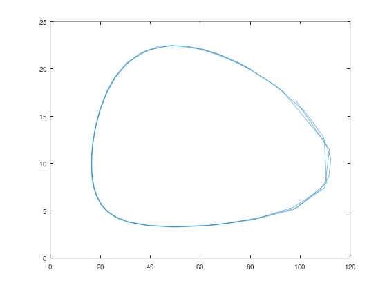
Figure 10.2 shows the result, which is called a phase plot. Each point on this plot represents a certain number of rabbits (on the x-axis) and a certain number of foxes (on the y-axis). Since these are the only two variables in the system, each point in this plane describes the complete state of the system, that is, the values of the variables we’re solving for.

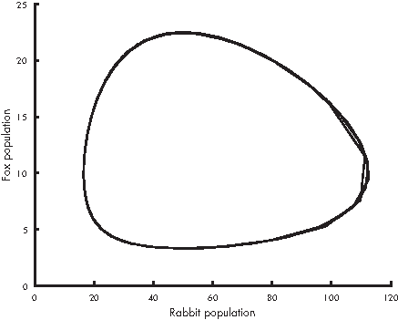
Figure 10.2: Phase plot from the Lotka-Volterra model

Over time, the state moves around the plane. Figure 10.2 shows the path traced by the state over time; this path is called a trajectory.

Since the behavior of this system is periodic, the trajectory is a loop.

If there are three variables in the system, we need three dimensions to show the state of the system, so the trajectory is a 3D curve. You can use plot3 to trace trajectories in three dimensions, but for four or more variables, you’re on your own.

What Could Go Wrong?

The output vector from the rate function has to be a column vector, otherwise you get an error:

In MATLAB, the error message is:

Error using odearguments (line 93)
RATE_FUNC must return a column vector.

In Octave, ode45 accepts a rate function that returns a row vector, so you don’t get this error; but return a column vector anyway, so your code works in MATLAB.

which is a pretty good error message. It’s not clear why it needs to be a column vector, but that’s not our problem.

Another possible error is reversing the order of the elements in the initial conditions or the vectors inside lotka. MATLAB doesn’t know what the elements are supposed to mean, so it can’t catch errors like this; it will just produce incorrect results.

The order of the elements (rabbits and foxes) is up to you, but you have to be consistent. That is, the order of the initial conditions you provide when you call ode45 has to be the same as the order inside rate_func where you unpack the input vector and the same as the order of the derivatives in the output vector.

Chapter Review

In this chapter, we used ode45 to solve a system of first-order differential equations. As an exercise, you’ll have a chance to solve the famous Lorenz equations, one of the first examples of a chaotic system.

Here are the terms from this chapter you might want to remember.

A row vector is a matrix that has only one row, and a column vector is a matrix that has only one column. The transpose operation transforms the rows of a matrix into columns (or the other way around, if you prefer).

A system of equations is a collection of equations written in terms of the same set of variables.

In a rate function, we often have to unpack the input variable, copying the elements of a vector into a set of variables. Then we have to pack the results into a vector as an output variable.

The state of a system is a set of variables that quantify the condition of the system as it changes over time.

When we solve a system of differential equations, we can visualize the results with a phase plot, which shows the state of a system as a point in the space of possible states. A trajectory is a path in a phase plot that shows how the state of a system changes over time.

In the next chapter, we’ll move on to second-order systems, which we use to describe systems with objects moving in space, governed by Newton’s laws of motion.

Exercises

Before you go on, you might want to work on the following exercise.

Exercise 10.2.

Based on the examples we’ve seen so far, you’d think that all ODEs describe population as a function of time, but that’s not true.

For example, the Lorenz system is a system of differential equations based on a model of fluid dynamics in the atmosphere (see https://greenteapress.com/matlab/lorenz). It turns out to be interesting in part because its solutions are chaotic; that is, small changes in the initial conditions yield big differences in the solutions.

The system is described by these differential equations:

\[\begin{split}\begin{aligned} x_t &= \sigma (y - x) \\ y_t &= x (r - z) - y \\ z_t &= xy - b z \end{aligned}\end{split}\]

Common values for the parameters are \(\sigma = 10\), \(b = 8/3\), and \(r=28\).

Use ode45 to estimate a solution to this system of equations.

1. Create a file named lorenz.m with a top-level function named lorenz and a helper function named rate_func.

2. The rate function should take t and V as input variables, where the components of V are understood to be the current values of x, y, and z. It should compute the corresponding derivatives and return them in a single column vector.

3. Test the function by calling it from the top-level function with values like \(t=0\), \(x=1\), \(y=2\), and \(z=3\). Once you get your function working, you should make it a silent function before calling ode45.

4. Use ode45 to estimate the solution for the time span \([0, 30]\) with the initial condition \(x=1\), \(y=2\), and \(z=3\).

5. Plot the results as a time series, that is, each of the variables as a function of time.

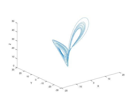
6. Use plot3 to plot the trajectory of \(x\), \(y\), and \(z\).

% Exercise 10.1 (the transpose operator): your solution here

Show solution

Hide solution

% Solution

% Solve the Lorentz system and plot the results.

function res = lorenz()
    % Run the ode solver
    [T, M] = ode45(@rate_func, [0 30], [1 2 3]);

    % plot the results
    X = M(:,1);
    Y = M(:,2);
    Z = M(:,3);
    plot3(X, Y, Z)
    xlabel('X')
    ylabel('Y')
    zlabel('Z')

    % uncomment this to see the trajectory animated
    % comet3(X, Y, Z);
end

function res = rate_func(t, V)
    % unpack the state vector
    x = V(1);
    y = V(2);
    z = V(3);

    % set the parameters
    sigma = 10;
    b = 8/3;
    r = 28;

    % compute the derivatives
    dxdt = sigma * (y-x);
    dydt = x * (r-z) - y;
    dzdt = x*y - b*z;

    % pack the results in a column vector
    res = [dxdt; dydt; dzdt];
end

Show solution

Hide solution

% Solution

lorenz