Notebook 3: Estimating Proportions¶

License: Attribution-NonCommercial-ShareAlike 4.0 International (CC BY-NC-SA 4.0)

# If we're running on Colab, install PyMC and ArviZ
import sys
IN_COLAB = 'google.colab' in sys.modules

if IN_COLAB:
    !pip install pymc3
    !pip install arviz

# PyMC generates a FutureWarning we don't need to deal with yet

import warnings
warnings.filterwarnings("ignore", category=FutureWarning)

import seaborn as sns

def plot_hist(sample, **options):
    """Plot a histogram of goals.
    
    sample: sequence of values
    """
    sns.histplot(sample, stat='probability', discrete=True,
                 alpha=0.5, **options)

def plot_kde(sample, **options):
    """Plot a distribution using KDE.
    
    sample: sequence of values
    """
    sns.kdeplot(sample, cut=0, **options)

import matplotlib.pyplot as plt

def legend(**options):
    """Make a legend only if there are labels."""
    handles, labels = plt.gca().get_legend_handles_labels()
    if len(labels):
        plt.legend(**options)

Estimating proportions¶

In Information Theory, Inference, and Learning Algorithms, David MacKay poses this problem:

“A statistical statement appeared in The Guardian on Friday January 4, 2002:

When spun on edge 250 times, a Belgian one-euro coin came up heads 140 times and tails 110. ‘It looks very suspicious to me,’ said Barry Blight, a statistics lecturer at the London School of Economics. ‘If the coin were unbiased, the chance of getting a result as extreme as that would be less than 7%.’

“But [MacKay asks] do these data give evidence that the coin is biased rather than fair?”

To answer that question, we’ll use the observed data to estimate the probability that the coin comes up heads.

But I’ll start with the binomial distribution.

Binomial distribution¶

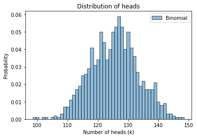
Suppose we know for sure that the coin is fair, that is, that the probability of heads is exactly 50%. If we spin it on edge 250 times, we expect the number of heads to follow a binomial distribution with parameters n=250 and p=0.5.

And we can use PyMC to generate a sample of values from that distribution.

n = 250
p = 0.5

import pymc3 as pm

sample_binomial = pm.Binomial.dist(n, p).random(size=1000)
sample_binomial.mean()

125.411

Here’s what the distribution of the sample looks like.

def decorate_heads(ylabel='Probability'):
    """Decorate the axes."""
    plt.xlabel('Number of heads (k)')
    plt.ylabel(ylabel)
    plt.title('Distribution of heads')
    legend()

plot_hist(sample_binomial, label='Binomial')
decorate_heads()

The beta distribution¶

In the previous section I assumed that the actual probability of heads is known, but in general it is not. And for the Euro problem, the probability of heads is what we would like to estimate.

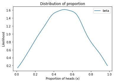
So, just as we used a gamma distribution to represent possible values for the goal scoring rate, mu, now we will use a beta distribution to represent possible values for the probability of heads, which I will call x.

The beta distribution is not the only possibility, but it is continuous and defined for values between 0 and 1 (including both) so it is appropriate for values that are probabilities.

The shape of the beta distribution is controlled by two parameters, called alpha and beta.

alpha = 2
beta = 2

And we can use PyMC to draw a sample from a beta distribution with given parameters.

sample_beta = pm.Beta.dist(alpha=alpha, beta=beta).random(size=1000)
sample_beta.mean()

0.5025838401365187

Here’s what the beta distribution looks like with alpha=2 and beta=2.

def decorate_proportion(ylabel='Likelihood'):
    """Decorate the axes."""
    plt.xlabel('Proportion of heads (x)')
    plt.ylabel(ylabel)
    plt.title('Distribution of proportion')
    legend()

plot_kde(sample_beta, label='beta')
decorate_proportion()

Exercise: See what the distribution looks like with different values of alpha and beta.

The Beta-Binomial model¶

To model the coin-spinning process, I’ll draw values of x from a beta distribution and then draw values of k from a binomial distribution.

Remember that x is the probability of heads, which is a continuous value between 0 and 1, and k is the number of heads, which is an integer between 0 and n.

Here’s what the model looks like in PyMC.

alpha = 2
beta = 2
n = 250

with pm.Model() as model1:
    x = pm.Beta('x', alpha=alpha, beta=alpha)
    k = pm.Binomial('k', n=n, p=x)
    trace1 = pm.sample_prior_predictive(1000)

The variables x and k are connected because the value of x is a parameter for the distribution of k.

Here’s the graphical representation that shows this connection.

pm.model_to_graphviz(model1)

From the trace we can extract x, which is a sample from the prior distribution.

sample_prior = trace1['x']
sample_prior.mean()

0.5032355465488882

Here’s what it looks like.

plot_kde(sample_prior)
decorate_proportion()

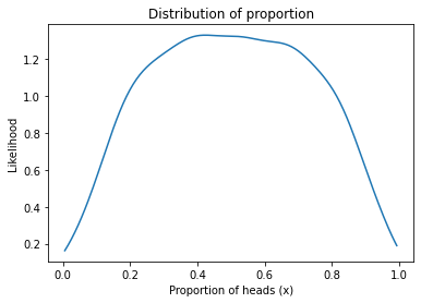
This distribution represents a belief about coins; specifically, it suggests that most coins are close to fair, with values of x between 0.4 and 0.6, but some coins are strongly biased, with values of x near 0 and 1.

In reality, I suspect that coins are not really as variable as this; I can imagine that x might be as low as 0.4 or as high as 0.6, but I would be surprised if it were much outside that range.

So this prior might not represent everything we know about coins, but in this example it turns out not to affect the result very much.

The prior predictive distribution¶

From the same trace we can extract k, which is the prior predictive distribution. It represents the number of heads we expect, with n=250, based on the prior distribution of x.

sample_prior_pred = trace1['k']
sample_prior_pred.mean()

125.891

Here’s what the distribution looks like.

plot_hist(sample_prior_pred, label='prior pred')
decorate_heads()

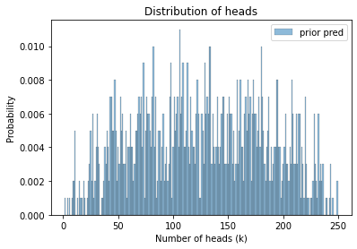
If we believe what the prior distribution says about x, this is what we should believe about k.

Now let’s use the data to update it.

Inference¶

From the previous model, it is a small change to draw a sample from the posterior distribution of x.

k_obs = 140

with pm.Model() as model2:
    x = pm.Beta('x', alpha=2, beta=2)
    k = pm.Binomial('k', n=n, p=x, observed=k_obs)
    trace2 = pm.sample(500)

Auto-assigning NUTS sampler...
Initializing NUTS using jitter+adapt_diag...
Multiprocess sampling (4 chains in 4 jobs)
NUTS: [x]

100.00% [6000/6000 00:01<00:00 Sampling 4 chains, 0 divergences]

Sampling 4 chains for 1_000 tune and 500 draw iterations (4_000 + 2_000 draws total) took 1 seconds.
The acceptance probability does not match the target. It is 0.8920679281335565, but should be close to 0.8. Try to increase the number of tuning steps.

The trace contains a sample of values from the posterior distribution of x.

len(trace2['x'])

We can use plot_trace to see if the sampler ran into any problems.

import arviz as az

with model2:
    az.plot_trace(trace2)

And plot_posterior to see the posterior distribution.

with model2:
    az.plot_posterior(trace2)

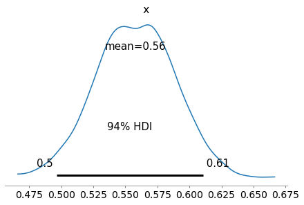
Again, the 94% HDI is a credible interval that have a 94% chance of containing the true value of x for this coin.

Exercise:

In this example, we are primarily interested in estimating x, but we can also use the posterior predictive distribution to predict what would happen if we spun the same coin again.

Use sample_posterior_predictive to generate a sample of k, then use plot_hist to plot the posterior predictive distribution.

Bayesian Inference with PyMC