Notebook 2: Making Predictions¶

License: Attribution-NonCommercial-ShareAlike 4.0 International (CC BY-NC-SA 4.0)

# If we're running on Colab, install PyMC and ArviZ
import sys
IN_COLAB = 'google.colab' in sys.modules

if IN_COLAB:
    !pip install pymc3
    !pip install arviz

# PyMC generates a FutureWarning we don't need to deal with yet

import warnings
warnings.filterwarnings("ignore", category=FutureWarning)

import seaborn as sns

def plot_hist(sample, **options):
    """Plot a histogram of goals.
    
    sample: sequence of values
    """
    sns.histplot(sample, stat='probability', discrete=True,
                 alpha=0.5, **options)

import matplotlib.pyplot as plt

def legend(**options):
    """Make a legend only if there are labels."""
    handles, labels = plt.gca().get_legend_handles_labels()
    if len(labels):
        plt.legend(**options)
        
def decorate_goals(ylabel='Probability'):
    """Decorate the axes."""
    plt.xlabel('Number of goals')
    plt.ylabel(ylabel)
    plt.title('Distribution of goals scored')
    legend()

def plot_kde(sample, **options):
    """Plot a distribution using KDE.
    
    sample: sequence of values
    """
    sns.kdeplot(sample, cut=0, **options)

def decorate_rate(ylabel='Likelihood'):
    """Decorate the axes."""
    plt.xlabel('Goals per game (mu)')
    plt.ylabel(ylabel)
    plt.title('Distribution of goal scoring rate')
    legend()

Prediction¶

In the previous notebook, we defined a model with a goal-scoring rate drawn from a gamma distribution and a number of goals drawn from a Poisson distribution.

We defined a prior distribution for the goal-scoring rate, mu, and computed the prior predictive distribution, which is the distribution of goals based on the prior distribution.

Then we used PyMC to draw a sample from the posterior distribution, which is what we believe about mu based on observed data. And we used a two-team model to compute the probability of superiority, which is the chance that one team is better than another – in the sense of having a higher goal-scoring rate – based on an observed outcome.

Now let’s turn to the task of prediction; that is, given what we believe about mu, what distribution of goals should we expect if the same teams play again. From that we can compute the probability that each team would win a rematch.

Here’s the one-team model from the previous notebook, again.

alpha = 4.6
beta = 1.9

import pymc3 as pm

with pm.Model() as model1:
    mu = pm.Gamma('mu', alpha, beta)
    goals = pm.Poisson('goals', mu, observed=4)
    trace1 = pm.sample(500)

Auto-assigning NUTS sampler...
Initializing NUTS using jitter+adapt_diag...
Multiprocess sampling (4 chains in 4 jobs)
NUTS: [mu]

100.00% [6000/6000 00:00<00:00 Sampling 4 chains, 0 divergences]

Sampling 4 chains for 1_000 tune and 500 draw iterations (4_000 + 2_000 draws total) took 1 seconds.
The acceptance probability does not match the target. It is 0.9052933922028723, but should be close to 0.8. Try to increase the number of tuning steps.

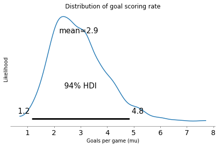
And here’s the posterior distribution of mu.

sample_posterior = trace1['mu']
len(sample_posterior)

import arviz as az

az.plot_posterior(sample_posterior)
decorate_rate()

Posterior predictive distribution¶

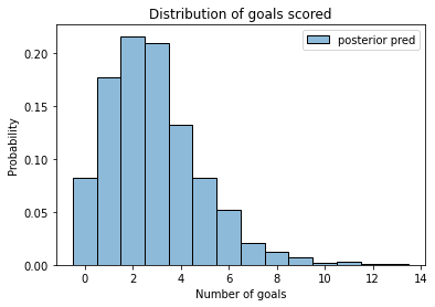
That tells us what we should believe about mu after we see the data, but it doesn’t tell us how many goals we should expect in the future. For that, we need the posterior predictive distribution, which we can get by running sample_posterior_predictive:

with model1:
    post_pred = pm.sample_posterior_predictive(trace1)

100.00% [2000/2000 00:00<00:00]

The result is similar to the trace we got from sample, but it contains a sample of goals rather than mu.

sample_post_pred = post_pred['goals']
sample_post_pred.mean()

2.8725

And here’s what it looks like.

plot_hist(sample_post_pred, label='posterior pred')
decorate_goals()

Two teams¶

Continuing the example from the previous notebook, suppose two teams have played each other twice, Team A wins the first game 5-1 and the second game 3-1. The following model computes the posterior distribution for each team based on these outcomes.

with pm.Model() as model2:
    mu_A = pm.Gamma('mu_A', alpha, beta)
    mu_B = pm.Gamma('mu_B', alpha, beta)
    goals_A = pm.Poisson('goals_A', mu_A, observed=[5,3])
    goals_B = pm.Poisson('goals_B', mu_B, observed=[1,1])
    trace2 = pm.sample(500)

Auto-assigning NUTS sampler...
Initializing NUTS using jitter+adapt_diag...
Multiprocess sampling (4 chains in 4 jobs)
NUTS: [mu_B, mu_A]

100.00% [6000/6000 00:00<00:00 Sampling 4 chains, 0 divergences]

Sampling 4 chains for 1_000 tune and 500 draw iterations (4_000 + 2_000 draws total) took 1 seconds.

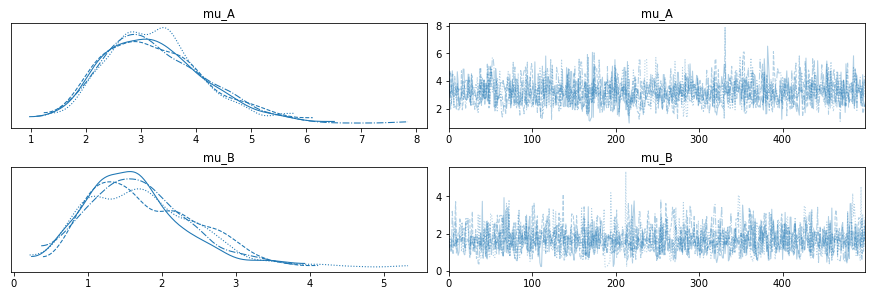
Here are the results.

import arviz as az

with model2:
    az.plot_trace(trace2);

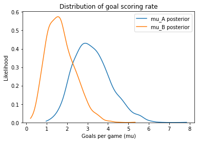
And here are the posterior distributions for mu_B and mu_A.

mu_A = trace2['mu_A']
mu_B = trace2['mu_B']
mu_B.mean(), mu_A.mean()

(1.6979206839296863, 3.2345281980077862)

plot_kde(mu_A, label='mu_A posterior')
plot_kde(mu_B, label='mu_B posterior')
decorate_rate()

And here’s the probability of superiority.

(mu_A > mu_B).mean()

0.921

Based on the results, we can be fairly confident that A is the better team, but that doesn’t necessarily mean they will win the next game.

Predictions¶

To compute the probability that A wins the next game, we can use sample_posterior_predictive to generate predictions.

with model2:
    post_pred = pm.sample_posterior_predictive(trace2)

100.00% [2000/2000 00:01<00:00]

The prediction for each is an array, so I’ll flatten it into a sequence.

goals_A = post_pred['goals_A']
goals_A.shape

(2000, 2)

Here are the posterior predictive distributions of goals scored.

goals_A = post_pred['goals_A'].flatten()
goals_B = post_pred['goals_B'].flatten()

plot_hist(goals_A, label='A')
plot_hist(goals_B, color='C1', label='B')
decorate_goals('PMF')

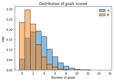
Team B is more likely than Team A to score 0, 1, or 2 goals. Team A is more likely to score 3 or more.

Here’s the chance that A wins the next game.

win = (goals_A > goals_B).mean()
win

0.6705

The chance that they lose.

lose = (goals_B > goals_A).mean()
lose

0.18525

And the chance of a tie.

tie = (goals_B == goals_A).mean()
tie

0.14425

Sudden death¶

In overtime, whichever team scores first wins. If we treat goal-scoring as a Poisson process, the time until the next goal is exponential with parameter 1/mu.

We can use the samples from the posterior distributions to generate samples from the posterior predictive distribution of time until the next goal, in units of games.

t_A = pm.Exponential.dist(mu_A).random(1000)
t_A.mean()

0.3406099892260252

t_B = pm.Exponential.dist(mu_B).random(1000)
t_B.mean()

0.7085185642938957

On average, we expect it to take longer for Team B to score. But the game isn’t decided by averages.

Exercise: Compute the probability that Team A wins in overtime, then compute their total probability of winning the next game.

Bonus exercise: What is their probability of winning at least 2 of the remaining 5 games in the series?

Hint: Use pm.Binomial.dist to draw a sample of wins from a binomial distribution with n=5 and p=prob_win.

Bayesian Inference with PyMC