Survey Data with Pandas and StatsModels#
Tutorial for PyCon 2025
Allen B. Downey
Click here to run this notebook on Colab.
import pandas as pd
import numpy as np
import matplotlib.pyplot as plt
import seaborn as sns
Show code cell content
# Configure Matplotlib

plt.rcParams["figure.figsize"] = 7, 3.5
plt.rcParams["figure.dpi"] = 75
plt.rcParams["axes.titlelocation"] = "left"
plt.rcParams["axes.spines.top"] = False
plt.rcParams["axes.spines.bottom"] = False
plt.rcParams["axes.spines.left"] = False
plt.rcParams["axes.spines.right"] = False
from os.path import basename, exists

def download(url):
    filename = basename(url)
    if not exists(filename):
        from urllib.request import urlretrieve
        local, _ = urlretrieve(url, filename)
        print('Downloaded ' + local)
def decorate(**options):
    """Decorate the current axes.

    Call decorate with keyword arguments like
    decorate(title='Title',
             xlabel='x',
             ylabel='y')

    The keyword arguments can be any of the axis properties
    https://matplotlib.org/api/axes_api.html
    """
    legend = options.pop("legend", True)
    loc = options.pop("loc", "best")

    # Pass options to Axis.set
    ax = plt.gca()
    ax.set(**options)

    # Add a legend if there are any labeled elements
    handles, labels = ax.get_legend_handles_labels()
    if handles and legend:
        ax.legend(handles, labels, loc=loc)

    # Tight layout is generally a good idea
    plt.tight_layout()
Data#
We will use data from the General Social Survey (GSS). The raw dataset is big, so I’ve prepared an extract, which the following cell downloads. The code to generate the extract is in this notebook.
# This dataset is prepared in the GssExtract repository

DATA_PATH = "https://github.com/AllenDowney/GssExtract/raw/main/data/interim/"

filename = "gss_extract_pacs_workshop.hdf"
download(DATA_PATH + filename)
Show code cell content
# Solution

gss = pd.read_hdf(filename, "gss")
gss.shape
(72390, 29)
Show code cell content
# Solution

gss.head()
| age | attend | ballot | class | cohort | degree | educ | fair | fear | goodlife | ... | region | relig | rincome | satfin | satjob | sex | srcbelt | trust | wtssall | year | |
|---|---|---|---|---|---|---|---|---|---|---|---|---|---|---|---|---|---|---|---|---|---|
| 0 | 24.0 | 1.0 | NaN | 3.0 | 1948.0 | 3.0 | 16.0 | 2.0 | NaN | NaN | ... | 1 | 1.0 | NaN | 1.0 | NaN | 1.0 | 5.0 | 1.0 | 1.3339 | 1972 |
| 1 | 33.0 | 2.0 | NaN | 2.0 | 1939.0 | 0.0 | 10.0 | 2.0 | NaN | NaN | ... | 1 | 2.0 | NaN | 3.0 | 2.0 | 1.0 | 1.0 | 1.0 | 0.8893 | 1972 |
| 2 | 40.0 | 8.0 | NaN | 2.0 | 1932.0 | 1.0 | 12.0 | 2.0 | NaN | NaN | ... | 1 | 5.0 | NaN | 1.0 | NaN | 2.0 | 3.0 | 2.0 | 1.3339 | 1972 |
| 3 | 24.0 | 2.0 | NaN | 2.0 | 1948.0 | 1.0 | 12.0 | 1.0 | NaN | NaN | ... | 9 | 2.0 | NaN | 2.0 | NaN | 1.0 | 3.0 | 2.0 | 1.7786 | 1972 |
| 4 | 21.0 | 7.0 | NaN | 3.0 | 1951.0 | 1.0 | 12.0 | 1.0 | NaN | NaN | ... | 9 | 1.0 | NaN | 1.0 | NaN | 2.0 | 2.0 | NaN | 1.7786 | 1972 |
5 rows × 29 columns
Show code cell content
# Solution

gss.columns
Index(['age', 'attend', 'ballot', 'class', 'cohort', 'degree', 'educ', 'fair',
       'fear', 'goodlife', 'hapmar', 'happy', 'health', 'helpful', 'id',
       'life', 'partyid', 'polviews', 'race', 'region', 'relig', 'rincome',
       'satfin', 'satjob', 'sex', 'srcbelt', 'trust', 'wtssall', 'year'],
      dtype='object')
Show code cell content
# Solution

gss.isna().mean().sort_values()
id          0.000000
year        0.000000
wtssall     0.000000
region      0.000000
srcbelt     0.000718
race        0.001796
sex         0.002086
degree      0.002942
educ        0.004338
cohort      0.005567
relig       0.007087
partyid     0.007294
attend      0.009711
age         0.010416
class       0.048501
satfin      0.063641
happy       0.065106
polviews    0.131620
health      0.236552
satjob      0.265064
ballot      0.302183
fear        0.365147
life        0.386669
rincome     0.402086
trust       0.410982
helpful     0.414090
fair        0.415665
hapmar      0.468241
goodlife    0.631924
dtype: float64
Distributions#
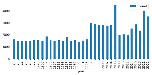
We’ll see two ways to describe distributions: value counts and KDE.
And for joint distributions, we’ll use a cross tabulation.
def value_counts(seq, **options):
    """Make a series of values and the number of times they appear.

    Args:
        seq: sequence

    returns: Pandas Series
    """
    return pd.Series(seq).value_counts(**options).sort_index()
Show code cell content
# Solution

pmf = value_counts(gss['year'])
pmf.plot(kind='bar')
decorate()
Show code cell content
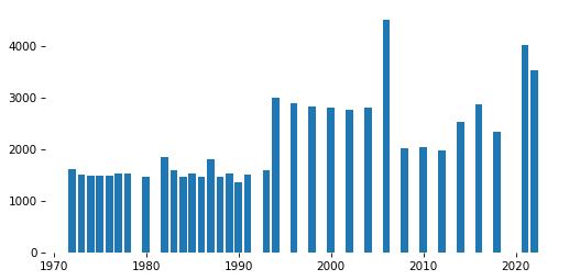
# Solution

x, y = pmf.index, pmf.values
plt.bar(x, y)
decorate()
Show code cell content
# Solution
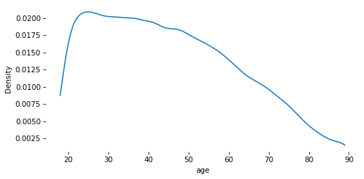
gss['age'].describe()
count    71636.000000
mean        44.985943
std         17.201666
min         18.000000
25%         30.000000
50%         43.000000
75%         58.000000
max         89.000000
Name: age, dtype: float64
Show code cell content
# Solution

sns.kdeplot(gss['age'], cut=0)
decorate()
Show code cell content
# Solution

gss['cohort'].describe()
count    71987.000000
mean      1991.908095
std        561.717010
min       1883.000000
25%       1938.000000
50%       1954.000000
75%       1968.000000
max       9999.000000
Name: cohort, dtype: float64
Show code cell content
# Solution

gss['cohort'] = gss['cohort'].replace(9999, np.nan)
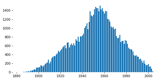
Exercise#
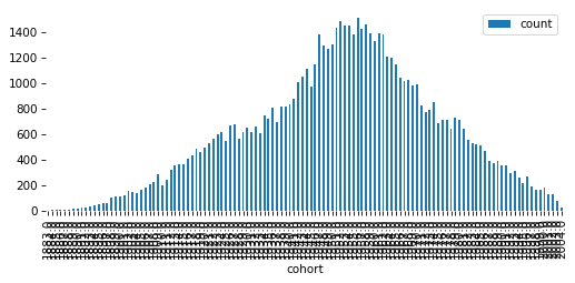
Use value_counts to plot the distribution of cohort as a bar plot.
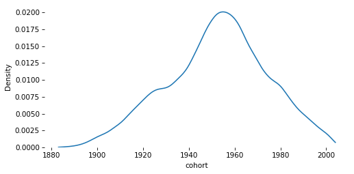
Then use sns.kdeplot to show the same distribution as a continuous quantity.
Show code cell content
# Solution

pmf = value_counts(gss['cohort'])
pmf.plot(kind='bar')
decorate(ylabel='Count')
Show code cell content
# Solution

x, y = pmf.index, pmf.values
plt.bar(x, y)
decorate(ylabel='Count')
Show code cell content
# Solution

sns.kdeplot(gss['cohort'], cut=0)
decorate()
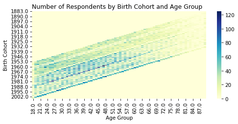
Cross tabulation#
Cross tabulation is a way to represent the joint distribution of two variables.
Show code cell content
# Solution

xtab = pd.crosstab(gss['cohort'], gss['age'])
xtab
| age | 18.0 | 19.0 | 20.0 | 21.0 | 22.0 | 23.0 | 24.0 | 25.0 | 26.0 | 27.0 | ... | 80.0 | 81.0 | 82.0 | 83.0 | 84.0 | 85.0 | 86.0 | 87.0 | 88.0 | 89.0 |
|---|---|---|---|---|---|---|---|---|---|---|---|---|---|---|---|---|---|---|---|---|---|
| cohort | |||||||||||||||||||||
| 1883.0 | 0 | 0 | 0 | 0 | 0 | 0 | 0 | 0 | 0 | 0 | ... | 0 | 0 | 0 | 0 | 0 | 0 | 0 | 0 | 0 | 1 |
| 1884.0 | 0 | 0 | 0 | 0 | 0 | 0 | 0 | 0 | 0 | 0 | ... | 0 | 0 | 0 | 0 | 0 | 0 | 0 | 0 | 1 | 1 |
| 1885.0 | 0 | 0 | 0 | 0 | 0 | 0 | 0 | 0 | 0 | 0 | ... | 0 | 0 | 0 | 0 | 0 | 0 | 0 | 0 | 0 | 5 |
| 1886.0 | 0 | 0 | 0 | 0 | 0 | 0 | 0 | 0 | 0 | 0 | ... | 0 | 0 | 0 | 0 | 0 | 0 | 0 | 0 | 4 | 4 |
| 1887.0 | 0 | 0 | 0 | 0 | 0 | 0 | 0 | 0 | 0 | 0 | ... | 0 | 0 | 0 | 0 | 0 | 2 | 1 | 0 | 1 | 4 |
| ... | ... | ... | ... | ... | ... | ... | ... | ... | ... | ... | ... | ... | ... | ... | ... | ... | ... | ... | ... | ... | ... |
| 2000.0 | 36 | 0 | 0 | 71 | 77 | 0 | 0 | 0 | 0 | 0 | ... | 0 | 0 | 0 | 0 | 0 | 0 | 0 | 0 | 0 | 0 |
| 2001.0 | 0 | 0 | 68 | 63 | 0 | 0 | 0 | 0 | 0 | 0 | ... | 0 | 0 | 0 | 0 | 0 | 0 | 0 | 0 | 0 | 0 |
| 2002.0 | 0 | 59 | 69 | 0 | 0 | 0 | 0 | 0 | 0 | 0 | ... | 0 | 0 | 0 | 0 | 0 | 0 | 0 | 0 | 0 | 0 |
| 2003.0 | 7 | 70 | 0 | 0 | 0 | 0 | 0 | 0 | 0 | 0 | ... | 0 | 0 | 0 | 0 | 0 | 0 | 0 | 0 | 0 | 0 |
| 2004.0 | 25 | 0 | 0 | 0 | 0 | 0 | 0 | 0 | 0 | 0 | ... | 0 | 0 | 0 | 0 | 0 | 0 | 0 | 0 | 0 | 0 |
122 rows × 72 columns
Show code cell content
# Solution

sns.heatmap(
    xtab,
    cmap="YlGnBu",
)

plt.title("Number of Respondents by Birth Cohort and Age Group")
plt.xlabel("Age Group")
plt.ylabel("Birth Cohort")
decorate()
Target variable#
I’ve selected four variables you might want to work with. Whichever one you choose, put its cell last.
# https://gssdataexplorer.norc.org/variables/434/vshow

varname = 'happy'

question = """Taken all together, how would you say things are these days--
would you say that you are very happy, pretty happy, or not too happy?
"""

responses = ['Very happy', "Happy", 'Not too happy']

ylabel = "Percent saying 'very happy'"
# https://gssdataexplorer.norc.org/variables/439/vshow

varname = 'helpful'

question = """Would you say that most of the time people try to be helpful,
or that they are mostly just looking out for themselves?
"""

responses = ['Helpful', 'Look out\nfor themselves', 'Depends']

ylabel = "Percent saying 'helpful'"
# https://gssdataexplorer.norc.org/variables/440/vshow

varname = 'fair'

question = """Do you think most people would try to take advantage of you
if they got a chance, or would they try to be fair?
"""

# notice that the negative response is first here!
responses = ['Take advantage', 'Fair', 'Depends']

ylabel = "Percent saying 'fair'"
# https://gssdataexplorer.norc.org/variables/441/vshow
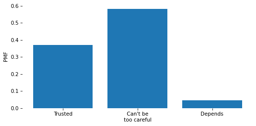
varname = 'trust'
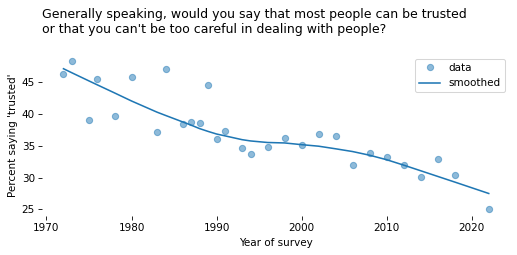
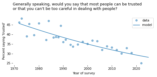
question = """Generally speaking, would you say that most people can be trusted
or that you can't be too careful in dealing with people?
"""
responses = ['Trusted', "Can't be\ntoo careful", 'Depends']
ylabel = "Percent saying 'trusted'"
Show code cell content
# Solution

column = gss[varname]
column
0        1.0
1        1.0
2        2.0
3        2.0
4        NaN
        ...
72385    2.0
72386    2.0
72387    NaN
72388    NaN
72389    1.0
Name: trust, Length: 72390, dtype: float64
Show code cell content
# Solution

value_counts(column, dropna=False)
trust
1.0    15783
2.0    24890
3.0     1966
NaN    29751
Name: count, dtype: int64
Show code cell content
# Solution
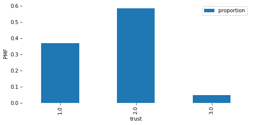
pmf = value_counts(column, normalize=True)
pmf
trust
1.0    0.370154
2.0    0.583738
3.0    0.046108
Name: proportion, dtype: float64
Show code cell content
# Solution

pmf.plot(kind='bar')
decorate(ylabel='PMF')
Show code cell content
# Solution

plt.bar(pmf.index, pmf)
plt.xticks(pmf.index, responses)

decorate(ylabel='PMF')
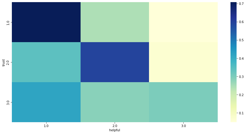
Exercise#
Do you think people who say “trust” are also more likely to say “helpful”?
To find out, make a cross tabulation of trust and helpful.
Consider using normalize='index'.
Make a heatmap that shows this joint distribution.
What relationships can you see in the responses?
Show code cell content
# Solution

xtab = pd.crosstab(gss['trust'], gss['helpful'], normalize='index')
xtab
| helpful | 1.0 | 2.0 | 3.0 |
|---|---|---|---|
| trust | |||
| 1.0 | 0.707773 | 0.243133 | 0.049094 |
| 2.0 | 0.340947 | 0.592560 | 0.066493 |
| 3.0 | 0.417197 | 0.283970 | 0.298832 |
Show code cell content
# Solution

plt.figure(figsize=(12, 6))
sns.heatmap(
    xtab,
    cmap="YlGnBu",
)

decorate(xlabel='helpful', ylabel='trust')
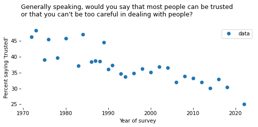
Time Series#
To see how responses have changed over time, we’ll use cross tabulation again.
Show code cell content
# Solution

xtab = pd.crosstab(gss["year"], gss[varname], normalize='index')
xtab.head()
| trust | 1.0 | 2.0 | 3.0 |
|---|---|---|---|
| year | |||
| 1972 | 0.463551 | 0.490343 | 0.046106 |
| 1973 | 0.483656 | 0.495664 | 0.020680 |
| 1975 | 0.391099 | 0.564396 | 0.044504 |
| 1976 | 0.455518 | 0.513043 | 0.031438 |
| 1978 | 0.396597 | 0.549738 | 0.053665 |
Show code cell content
# Solution

gss72 = gss.query('year == 1972')
gss72.shape
(1613, 29)
Show code cell content
# Solution

pmf72 = value_counts(gss72[varname], normalize=True)
pmf72
trust
1.0    0.463551
2.0    0.490343
3.0    0.046106
Name: proportion, dtype: float64
Show code cell content
# Solution

time_series = xtab[1] * 100
time_series.name = "data"
Show code cell content
# Solution

time_series.plot(style='o')
decorate(
    xlabel="Year of survey",
    ylabel=ylabel,
    title=question,
)
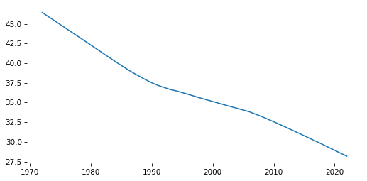
Smoothing#
To smooth the time series, we’ll use LOWESS (locally weighted scatterplot smoothing).
Show code cell content
# Solution

x = time_series.index.to_numpy()
y = time_series.to_numpy()
Show code cell content
# Solution

from statsmodels.nonparametric.smoothers_lowess import lowess

smooth_array = lowess(y, x)
Show code cell content
# Solution

index, data = np.transpose(smooth_array)
smooth_series = pd.Series(data, index=index)
Show code cell content
# Solution

smooth_series.plot()
decorate()
def make_lowess(series, frac=0.5):
    """Use LOWESS to compute a smooth line.

    series: pd.Series

    returns: pd.Series
    """
    y = series.to_numpy()
    x = series.index.to_numpy()

    smooth_array = lowess(y, x, frac)
    index, data = np.transpose(smooth_array)

    return pd.Series(data, index=index)
Exercise#
Use this function to make smooth_series.
Plot the result along with time_series.
Show code cell content
# Solution

smooth_series = make_lowess(time_series)
Show code cell content
# Solution

time_series.plot(style='o', alpha=0.5)
smooth_series.plot(label='smoothed', color='C0')

decorate(
    xlabel="Year of survey",
    ylabel=ylabel,
    title=question,
)
Binary series#
It will be useful to convert the responses to a binary variable represented with 0s and 1s.
Show code cell content
# Solution

# tempting but wrong

gss['y'] = gss[varname] == 1
value_counts(gss['y'], dropna=False)
y
False    56607
True     15783
Name: count, dtype: int64
Show code cell content
# Solution

gss['y'] = np.where(gss[varname].notna(), gss[varname] == 1, np.nan)
value_counts(gss['y'], dropna=False)
y
0.0    26856
1.0    15783
NaN    29751
Name: count, dtype: int64
Show code cell content
# Solution

# Reminder: this needs to be updated depending on the target variable

gss['y'] = gss[varname].replace([1, 2, 3], [1, 0, 0])
value_counts(gss['y'], dropna=False)
y
0.0    26856
1.0    15783
NaN    29751
Name: count, dtype: int64
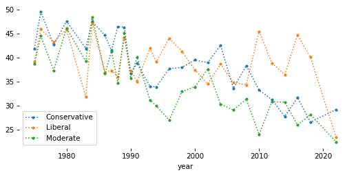
Pivot tables#
Now we’ll use a pivot table to put respondents in groups and see how the responses have changed over time.
polviews_map = {
    1: 'Liberal',
    2: 'Liberal',
    3: 'Liberal',
    4: 'Moderate',
    5: 'Conservative',
    6: 'Conservative',
    7: 'Conservative',
}
Show code cell content
# Solution

gss['polviews3'] = gss['polviews'].replace(polviews_map)
Show code cell content
# Solution

value_counts(gss['polviews3'], dropna=False)
polviews3
Conservative    21580
Liberal         17370
Moderate        23912
NaN              9528
Name: count, dtype: int64
Show code cell content
# Solution

table = gss.pivot_table(
    index='year', columns='polviews3', values='y', aggfunc='mean'
) * 100
table.head()
| polviews3 | Conservative | Liberal | Moderate |
|---|---|---|---|
| year | |||
| 1975 | 41.891892 | 39.192399 | 38.733706 |
| 1976 | 49.590164 | 45.961003 | 44.561404 |
| 1978 | 42.699115 | 43.262411 | 37.347295 |
| 1980 | 47.609562 | 45.896657 | 46.204620 |
| 1983 | 41.935484 | 31.914894 | 39.240506 |
Show code cell content
# Solution

table.plot(style='.:')
decorate()
Better colors#
We’ll select colors from a Seaborn color palette.
Show code cell content
# Solution

muted = sns.color_palette('muted', 5)
sns.palplot(muted)
Show code cell content
# Solution

color_map = {
    'Conservative': muted[3],
    'Moderate': muted[4],
    'Liberal': muted[0]
}
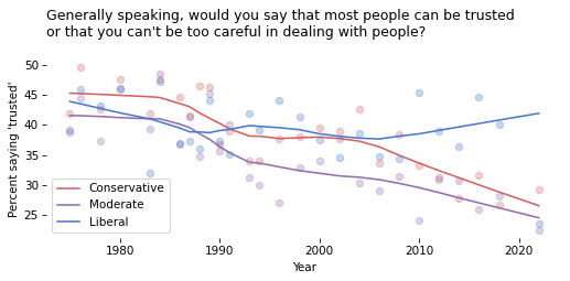
Exercise#
Loop through the groups in color_map.
For each one, extract a column from table and plot the data points; then plot a smooth line.
Show code cell content
# Solution

for group in color_map:
    series = table[group]
    color = color_map[group]
    series.plot(style='o', label='', color=color, alpha=0.3)
    smooth = make_lowess(series)
    smooth.plot(label=group, color=color)

decorate(
    xlabel='Year',
    ylabel=ylabel,
    title=question,
)
Groupby#
Now that we have y as a binary variable, we have another way to compute the time series and the pivot table.
There are pros and cons of each method.
Show code cell content
# Solution

valid = gss.dropna(subset=['y'])
Show code cell content
# Solution

time_series2 = valid.groupby('year')['y'].mean() * 100
assert np.allclose(time_series, time_series2)
Show code cell content
# Solution

table2 = valid.groupby(['year', 'polviews3'])['y'].mean().unstack() * 100
assert np.allclose(table, table2)
Logistic regression#
We’ll use logistic regression to model changes over time.
Show code cell content
# Solution

year_shift = gss['year'].median()
gss['x'] = gss['year'] - year_shift
Show code cell content
# Solution

subset = gss.dropna(subset=['y', 'x'])
Show code cell content
# Solution

import statsmodels.formula.api as smf

formula = 'y ~ x + I(x**2)'

model = smf.logit(formula, data=subset).fit(disp=False)
model.params
Intercept   -0.588941
x           -0.014565
I(x ** 2)    0.000057
dtype: float64
Show code cell content
# Solution

year_range = np.arange(1972, 2026)

pred_df = pd.DataFrame(dict(x=year_range - year_shift))

pred_series = model.predict(pred_df) * 100
pred_series.index = year_range
Show code cell content
# Solution

time_series.plot(style='o', alpha=0.5)
pred_series.plot(label='model', color='C0')

decorate(
    xlabel="Year of survey",
    ylabel=ylabel,
    title=question,
)
def fit_model(data, x_range, x_shift):
    formula = 'y ~ x + I(x**2)'
    model = smf.logit(formula, data=data).fit(disp=False)

    pred_df = pd.DataFrame(dict(x=x_range - x_shift))
    pred = model.predict(pred_df) * 100
    pred.index = x_range
    pred.name = 'model'

    return pred
Show code cell content
# Solution

pred_series2 = fit_model(subset, year_range, year_shift)
assert np.allclose(pred_series, pred_series2)
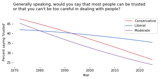
Exercise#
Use subset.groupby('polviews3') to loop through the groups.
For each one, use fit_model to generate and plot a “prediction” for the group.
Show code cell content
# Solution

for name, group in subset.groupby('polviews3'):
    pred_series = fit_model(group, year_range, year_shift)
    pred_series.plot(label=name, color=color_map[name])

decorate(
    xlabel='Year',
    ylabel=ylabel,
    title=question,
)
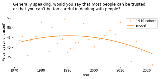
Group by cohort#
Now let’s group respondents by decade of birth and see how each cohort changes over time.
def round_into_bins(series, bin_width, low=0, high=None):
    """Rounds values down to the bin they belong in.

    series: pd.Series
    bin_width: number, width of the bins

    returns: Series of bin values (with NaN preserved)
    """
    if high is None:
        high = series.max()

    bins = np.arange(low, high + bin_width, bin_width)
    indices = np.digitize(series, bins)
    result = pd.Series(bins[indices - 1], index=series.index, dtype='float')

    result[series.isna()] = np.nan
    return result
Show code cell content
# Solution

gss["cohort10"] = round_into_bins(gss["cohort"], 10, 1880)
value_counts(gss["cohort10"], dropna=False)
cohort10
1880.0       45
1890.0      501
1900.0     1722
1910.0     3616
1920.0     5862
1930.0     7115
1940.0    10925
1950.0    14273
1960.0    11699
1970.0     7681
1980.0     5088
1990.0     2563
2000.0      545
NaN         755
Name: count, dtype: int64
Show code cell content
# Solution

cohort_df = gss.query("cohort10 == 1940").dropna(subset=['y', 'x'])
cohort_df.shape
(6825, 33)
Show code cell content
# Solution

cohort_series = cohort_df.groupby('year')['y'].mean() * 100
cohort_series.name = '1940 cohort'
Show code cell content
# Solution

x_range = cohort_series.index
pred_series = fit_model(cohort_df, x_range, year_shift)
Show code cell content
# Solution

cohort_series.plot(style='.', color='C1', alpha=0.5)
pred_series.plot(color='C1')

decorate(
    xlabel="Year",
    ylabel=ylabel,
    title=question,
)
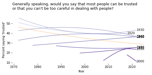
All the Cohorts#
Now let’s compare cohorts. The following function encapsulates the steps from the previous section.
def plot_cohort(df, cohort, color='C0'):
    cohort_df = df.query("cohort10 == @cohort").dropna(subset=['y', 'x'])

    cohort_series = cohort_df.groupby('year')['y'].mean() * 100

    year_range = cohort_series.index

    pred_series = fit_model(cohort_df, year_range, year_shift)
    x, y = pred_series.index[-1], pred_series.values[-1]
    plt.text(x, y, cohort, ha='left', va='center')

    pred_series.plot(label=cohort, color=color)
Show code cell content
# Solution

first, last = 1920, 2000
subset = gss.query("@first <= cohort <= @last" )
subset.shape
(65390, 33)
Show code cell content
# Solution

pred_all = fit_model(subset, year_range, year_shift)
Show code cell content
# Solution

cohorts = np.sort(subset['cohort10'].unique().astype(int))
cohorts
array([1920, 1930, 1940, 1950, 1960, 1970, 1980, 1990, 2000])
Show code cell content
# Solution

cmap = plt.get_cmap('Purples')

colors = [cmap(x) for x in np.linspace(0.3, 0.9, len(cohorts))]
Exercise#
Plot pred_all.
Then loop through cohorts and colors, and call plot_cohort for each group.
Depending on which target variable you chose, you might get a warning from StatsModels.
Show code cell content
# Solution

pred_all.plot(ls=':', color='C1')

for cohort, color in zip(cohorts, colors):
    plot_cohort(gss, cohort, color)

decorate(
    xlabel="Year",
    ylabel=ylabel,
    title=question,
    legend=False
)
/home/downey/miniconda3/envs/SurveyDataPandas/lib/python3.13/site-packages/statsmodels/base/model.py:607: ConvergenceWarning: Maximum Likelihood optimization failed to converge. Check mle_retvals
  warnings.warn("Maximum Likelihood optimization failed to "
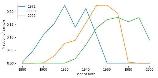
Simpson’s Paradox#
The composition of the population changes over time.
Show code cell content
# Solution

xtab_cohort = pd.crosstab(gss["cohort10"], gss["year"], normalize="columns")
xtab_cohort.head()
| year | 1972 | 1973 | 1974 | 1975 | 1976 | 1977 | 1978 | 1980 | 1982 | 1983 | ... | 2004 | 2006 | 2008 | 2010 | 2012 | 2014 | 2016 | 2018 | 2021 | 2022 |
|---|---|---|---|---|---|---|---|---|---|---|---|---|---|---|---|---|---|---|---|---|---|
| cohort10 | |||||||||||||||||||||
| 1880.0 | 0.003113 | 0.003995 | 0.008108 | 0.006739 | 0.004692 | 0.000000 | 0.003277 | 0.000000 | 0.000000 | 0.000000 | ... | 0.000000 | 0.000000 | 0.000000 | 0.000000 | 0.000000 | 0.000000 | 0.000000 | 0.000000 | 0.0 | 0.0 |
| 1890.0 | 0.047945 | 0.038615 | 0.029730 | 0.037062 | 0.047587 | 0.027613 | 0.028834 | 0.017088 | 0.018929 | 0.005013 | ... | 0.000000 | 0.000000 | 0.000000 | 0.000000 | 0.000000 | 0.000000 | 0.000000 | 0.000000 | 0.0 | 0.0 |
| 1900.0 | 0.110212 | 0.099201 | 0.129730 | 0.082210 | 0.070375 | 0.091387 | 0.083224 | 0.059467 | 0.051379 | 0.038221 | ... | 0.000000 | 0.000000 | 0.000000 | 0.000000 | 0.000000 | 0.000000 | 0.000000 | 0.000000 | 0.0 | 0.0 |
| 1910.0 | 0.152553 | 0.158455 | 0.131081 | 0.130728 | 0.144772 | 0.125575 | 0.105505 | 0.124402 | 0.103840 | 0.093358 | ... | 0.015714 | 0.007562 | 0.007944 | 0.000000 | 0.000000 | 0.000000 | 0.000000 | 0.000000 | 0.0 | 0.0 |
| 1920.0 | 0.224782 | 0.180426 | 0.193243 | 0.187332 | 0.159517 | 0.184747 | 0.152687 | 0.160629 | 0.149270 | 0.137218 | ... | 0.038929 | 0.040036 | 0.038232 | 0.035294 | 0.025381 | 0.014235 | 0.009807 | 0.008576 | 0.0 | 0.0 |
5 rows × 34 columns
Show code cell content
# Solution

xtab_cohort[1972].plot(label="1972")
xtab_cohort[1998].plot(label="1998")
xtab_cohort[2022].plot(label="2022")

decorate(xlabel="Year of birth", ylabel="Fraction of sample")
Sampling weights#
The GSS uses stratified sampling, so some respondents represent more people in the population than others. We can use resampling to correct for stratified sampling.
Show code cell content
# Solution

gss['wtssall'].describe()
count    72390.000000
mean         1.303960
std          0.889990
min          0.113721
25%          0.918400
50%          1.062700
75%          1.547800
max         14.272462
Name: wtssall, dtype: float64
Show code cell content
# Solution

gss.groupby('year')['wtssall'].describe()
| count | mean | std | min | 25% | 50% | 75% | max | |
|---|---|---|---|---|---|---|---|---|
| year | ||||||||
| 1972 | 1613.0 | 1.146481 | 0.486191 | 0.444600 | 0.889300 | 0.889300 | 1.333900 | 3.557100 |
| 1973 | 1504.0 | 1.130645 | 0.417802 | 0.457200 | 0.914500 | 0.914500 | 1.371700 | 2.743500 |
| 1974 | 1484.0 | 1.160032 | 0.443681 | 0.466000 | 0.932000 | 0.932000 | 1.397900 | 3.727900 |
| 1975 | 1490.0 | 1.140258 | 0.466167 | 0.466000 | 0.932000 | 0.932000 | 1.397900 | 3.261900 |
| 1976 | 1499.0 | 1.147392 | 0.459938 | 0.485400 | 0.970900 | 0.970900 | 1.456300 | 3.398100 |
| 1977 | 1530.0 | 1.161231 | 0.458057 | 0.494100 | 0.988100 | 0.988100 | 1.482200 | 2.964400 |
| 1978 | 1532.0 | 1.148797 | 0.448502 | 0.506300 | 1.012700 | 1.012700 | 1.519000 | 3.038000 |
| 1980 | 1468.0 | 1.168663 | 0.486058 | 0.511200 | 1.022500 | 1.022500 | 1.533700 | 3.578700 |
| 1982 | 1860.0 | 1.189170 | 0.513264 | 0.506400 | 1.031900 | 1.031900 | 1.547800 | 4.127500 |
| 1983 | 1599.0 | 1.174535 | 0.489286 | 0.505800 | 1.011600 | 1.011600 | 1.517500 | 3.540700 |
| 1984 | 1473.0 | 1.163876 | 0.473032 | 0.516500 | 1.033100 | 1.033100 | 1.549600 | 3.615700 |
| 1985 | 1534.0 | 1.158889 | 0.463941 | 0.518100 | 1.036300 | 1.036300 | 1.554400 | 3.626900 |
| 1986 | 1470.0 | 1.164447 | 0.467082 | 0.503600 | 1.007200 | 1.007200 | 1.510800 | 3.021600 |
| 1987 | 1819.0 | 1.186371 | 0.499286 | 0.505200 | 1.010400 | 1.010400 | 1.515500 | 3.536200 |
| 1988 | 1481.0 | 1.163860 | 0.463531 | 0.531300 | 1.062700 | 1.062700 | 1.062700 | 3.719400 |
| 1989 | 1537.0 | 1.184300 | 0.504330 | 0.510700 | 1.021500 | 1.021500 | 1.532200 | 3.575100 |
| 1990 | 1372.0 | 1.161439 | 0.489095 | 0.531300 | 1.062700 | 1.062700 | 1.062700 | 3.188100 |
| 1991 | 1517.0 | 1.174147 | 0.478842 | 0.531100 | 1.062100 | 1.062100 | 1.593200 | 3.717500 |
| 1993 | 1606.0 | 1.169310 | 0.448682 | 0.528500 | 1.057100 | 1.057100 | 1.585600 | 3.699800 |
| 1994 | 2992.0 | 1.166058 | 0.457253 | 0.541200 | 1.082500 | 1.082500 | 1.082500 | 3.247500 |
| 1996 | 2904.0 | 1.181024 | 0.479229 | 0.543200 | 1.086400 | 1.086400 | 1.086400 | 3.259100 |
| 1998 | 2832.0 | 1.177809 | 0.462729 | 0.550100 | 1.100100 | 1.100100 | 1.100100 | 3.850400 |
| 2000 | 2817.0 | 1.165950 | 0.453726 | 0.549300 | 1.098500 | 1.098500 | 1.098500 | 3.295600 |
| 2002 | 2765.0 | 1.198505 | 0.507470 | 0.557800 | 1.115600 | 1.115600 | 1.115600 | 2.788900 |
| 2004 | 2812.0 | 1.299424 | 0.762699 | 0.459200 | 0.918400 | 0.961700 | 1.836800 | 6.428700 |
| 2006 | 4510.0 | 1.360152 | 0.841060 | 0.429700 | 0.859300 | 0.954800 | 1.909600 | 5.728800 |
| 2008 | 2023.0 | 1.425750 | 0.911863 | 0.437745 | 0.875490 | 1.067670 | 2.135340 | 6.406021 |
| 2010 | 2044.0 | 1.313222 | 0.726111 | 0.463128 | 0.926255 | 0.926255 | 1.684101 | 4.210252 |
| 2012 | 1974.0 | 1.366495 | 0.884637 | 0.411898 | 0.823796 | 1.235694 | 1.747975 | 8.739876 |
| 2014 | 2538.0 | 1.273430 | 0.674193 | 0.448002 | 0.896003 | 1.344005 | 1.380591 | 5.376020 |
| 2016 | 2867.0 | 1.227412 | 0.607020 | 0.391825 | 0.956994 | 0.956994 | 1.564363 | 4.306471 |
| 2018 | 2348.0 | 1.382192 | 0.936160 | 0.471499 | 0.942997 | 0.942997 | 1.414496 | 5.897420 |
| 2021 | 4032.0 | 1.551637 | 1.175611 | 0.227357 | 0.790829 | 1.195842 | 1.869697 | 7.557038 |
| 2022 | 3544.0 | 2.551821 | 2.489079 | 0.113721 | 0.714314 | 1.781121 | 3.529911 | 14.272462 |
def resample_by_year(df, column='wtssall'):
    """Resample rows within each year using weighted sampling.

    df: DataFrame
    column: string name of weight variable

    returns: DataFrame
    """
    grouped = df.groupby('year')
    samples = [group.sample(n=len(group), replace=True, weights=group[column])
               for _, group in grouped]
    sample = pd.concat(samples, ignore_index=True)
    return sample
Show code cell content
# Solution

sample = resample_by_year(gss)
Show code cell content
# Solution

sample['y'].mean()
np.float64(0.36038778568752344)
Show code cell content
# Solution

gss['y'].mean()
np.float64(0.3701540842890312)
Show code cell content
# Solution

weighted_mean = np.average(valid['y'], weights=valid['wtssall'])
Copyright 2025 Allen Downey
The code in this notebook is under the MIT license.