This notebook contains the model presented in a talk at PyData Boston 2025.
Title: The SAT Math Gap: Gender Difference or Selection Bias?
Abstract
Why do male test takers consistently score about 30 points higher than female test takers on the mathematics section of the SAT? Does this reflect an actual difference in math ability, or is it an artifact of selection bias—if young men with low math ability are less likely to take the test than young women with the same ability?
This talk presents a Bayesian model that estimates how much of the observed difference can be explained by selection effects. We will walk through a complete Bayesian workflow, including prior elicitation with PreliZ, model building in PyMC, and validation with ArviZ, showing how Bayesian methods disentangle latent traits from observed outcomes and separate signal from noise.
No prior knowledge of Bayesian statistics is required; attendees should be familiar with Python and common probability distributions.
Overview
For decades, male test takers have outperformed female test takers on the SAT math section by about 30 points. This outcome could reflect a real difference in ability, or it could be explained by selection bias if boys with weaker math skills are less likely to take the SAT than girls with comparable skills.
I present a generative Bayesian model that explicitly incorporates this selection mechanism and estimates the fraction of the observed gap attributable to bias. The talk emphasizes workflow over theory: how to build, validate, and interpret Bayesian models using PyMC, ArviZ, and PreliZ.
Setup
On Colab, install the packages that aren’t in Colab’s Python. The pins keep the stack on PyMC 5 and ArviZ 0.x, the versions this analysis was run with: newer nutpie and PreliZ would upgrade them and break Colab’s PyMC.
import sys

if "google.colab" in sys.modules:
    %pip install -q nutpie "pymc<6" "arviz<1" "preliz==0.20.*" "matplotlib<3.11" empiricaldist
import pandas as pd
import numpy as np
import matplotlib.pyplot as plt
import os
os.makedirs("figs", exist_ok=True)
import pymc as pm
import arviz as az
import preliz as pz
import xarray as xr
import pytensor.tensor as pt
from scipy.special import expit
# NumPy 2.0 is annoying
np.set_printoptions(legacy='1.25')# Make the figures smaller to save some screen real estate
plt.rcParams["figure.dpi"] = 75
plt.rcParams["figure.figsize"] = [6, 3.5]def decorate(**options):
legend = options.pop("legend", True)
loc = options.pop("loc", "best")
ax = plt.gca()
ax.set(**options)
handles, labels = ax.get_legend_handles_labels()
if handles and legend:
ax.legend(handles, labels, loc=loc)
plt.tight_layout()SAT Data
Boys who take the SAT get higher math scores than girls, and the difference is consistent. In data published by the College Board for 2011-2015, the differences were 31, 34, 32, 31, and 31 points.
Reasons for this difference are a topic of debate. They include
Boys are better at math, on average.
Boys are better at taking the SAT, so the difference in scores overstates the difference in efficacy.
Boys who are bad at math are less likely to take the SAT than girls with the same efficacy -- due to this selection bias, the difference in scores overstates the difference in efficacy.
These articles are examples of the debate:
Mark J. Perry asserts that “2016 SAT Test Results Confirm Pattern That’s Persisted for 50 Years — High School Boys Are Better at Math Than Girls”.
Wendy Morrison and Grace Finley contend, “Actually, SAT Results Don’t Confirm Boys Are Better at Math Than Girls”, and they offer alternative explanations for the difference in scores.
And Perry responds, “Actually, 50 Years of Test Scores DO Confirm That Boys Outperform Girls on the SAT Math Test”, and explains why he finds the argument for a selection effect unconvincing.
If it’s true that boys with low math efficacy are less likely to take the SAT, we should see evidence of this effect in the distributions of scores, and we may be able to estimate the magnitude of the effect, and what fraction of the difference in scores we observe.
As data, we’ll use distributions of scores reported here:
2011 math: https://
Data for the writing section, and composite scores are also available for some years
2011 writing: https://
2011 composite: https://
2011 reading+math: https://
2012 reading: https://
2012 composite: https://
2012 reading+math: https://
2013 composite: https://
2013 reading+math https://
We used a PDF parser to extract the data from the PDF files. The results are available to download in a Zip file.
from os.path import basename, exists

def download(url):
    filename = basename(url)
    if not exists(filename):
        from urllib.request import urlretrieve

        local, _ = urlretrieve(url, filename)
        print("Downloaded " + local)

zip_filename = 'sat_math_csv_files.zip'
download('https://github.com/AllenDowney/SelectionSAT/raw/main/' + zip_filename)
import zipfile
if not exists('sat_math_2011.csv'):
with zipfile.ZipFile(zip_filename, 'r') as zip_ref:
zip_ref.extractall('.')
print(f"Extracted files: {', '.join(zip_ref.namelist())}")And use the following function to read them.
def read_sat_math(year):
    df = pd.read_csv(f'sat_math_{year}.csv', index_col=0)
    df.columns = ['Total', 'Male', 'Female']
    return df
The following dictionary maps from each year (2011-2015) to a Pandas DataFrame.
df_map = {}
years = range(2011, 2016)
for year in years:
    df_map[year] = read_sat_math(year)
Here are the total number of test takers in each year.
df_map[2011].sum()Total 1647123
Male 770605
Female 876518
dtype: int64df_map[2012].sum()Total 1664479
Male 778142
Female 886337
dtype: int64df_map[2013].sum()Total 1660047
Male 776092
Female 883955
dtype: int64df_map[2014].sum()Total 1672395
Male 783570
Female 888825
dtype: int64df_map[2015].sum()Total 1698521
Male 794802
Female 903719
dtype: int64In every year, substantially more girls than boys took the SAT, which is evidence that the selection effect is stronger for boys.
TODO: Get data on the number of boys and girls alive at test-taking age and the number who were enrolled in high school.
The following function converts the number of test-takers with each score into a normalized PMF.
from empiricaldist import Pmf

def make_pmf(df, col):
    pmf = Pmf(df[col])
    pmf.normalize()
    return pmf
Comparing the distribution of scores across years, we can see that the location and spread of the distributions appears consistent.
for year, df in df_map.items():
    pmf = make_pmf(df, 'Male')
    pmf.plot(label=year)

decorate(title='Male test-takers')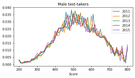
And likewise for female test takers.
for year, df in df_map.items():
    pmf = make_pmf(df, 'Female')
    pmf.plot(label=year)

decorate(title='Female test-takers')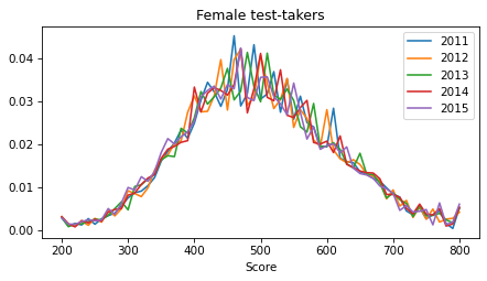
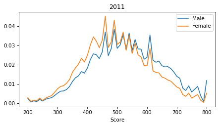
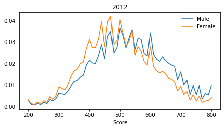
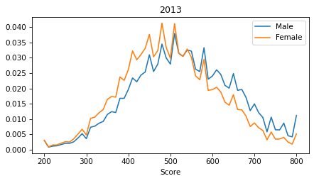
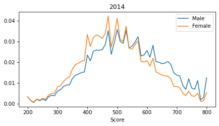
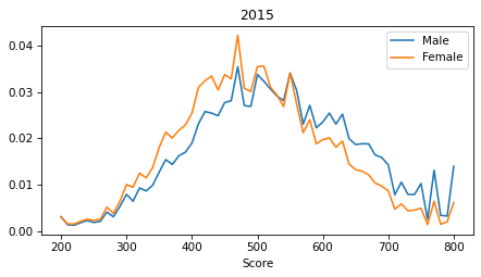
It is notable that the distributions are spiky. These perturbations are the result of the way SAT scores are computed. During 2011-2015 the math section of the SAT typically had 44 multiple choice questions and 10 grid questions. For the multiple-choice questions, incorrect answers were penalized by 1/4 point. In each year, some combinations of correct, incorrect, and blank responses were more likely than others. As a result, the PMF for each year shows a pattern of perturbations that is consistent for male and female test-takers, as shown in the following plots.
def compare_spikes(df_map, year):
    pmf_male = make_pmf(df_map[year], 'Male')
    pmf_male.plot(label='Male')

    pmf_female = make_pmf(df_map[year], 'Female')
    pmf_female.plot(label='Female')

    mean_male = pmf_male.mean()
    mean_female = pmf_female.mean()
    print(f'Male={mean_male}, Female={mean_female}, Diff={mean_male - mean_female}')
    decorate(title=year)
compare_spikes(df_map, 2011)Male=531.0491886245221, Female=499.6034993006419, Diff=31.44568932388023
compare_spikes(df_map, 2012)Male=532.3130225588645, Female=498.5023529425038, Diff=33.81066961636071
compare_spikes(df_map, 2013)Male=530.910871391536, Female=499.4024808955207, Diff=31.508390496015352
compare_spikes(df_map, 2014)Male=529.823844710747, Female=498.5317582201221, Diff=31.292086490624968
compare_spikes(df_map, 2015)Male=527.1939174788187, Female=495.92306900706967, Diff=31.27084847174899
It is also notable that the extreme scores (200 and 800) are overrepresented, which suggests that test scores don’t reflect the full range of efficacy.
years = [2011, 2012, 2013, 2014, 2015]
sexes = ['Male', 'Female']

rows = []
for year in years:
    for sex in sexes:
        df = df_map[year]
        pmf = make_pmf(df, sex)
        rows.append((year, sex, pmf.mean(), pmf.std()))

summary = pd.DataFrame(rows, columns=['Year', 'Sex', 'Mean', 'Std'])
We’ll use the following function later to plot the relationship between a potential score and the probability of taking the SAT.
def plot_selection_function(idata, thetas_scaled, **options):
    thetas_xr = xr.DataArray(thetas_scaled, dims="theta", coords={"theta": thetas})

    # Extract posterior samples of alpha and beta ---
    posterior = idata.posterior  # shape (chain, draw)

    # Compute logits and apply sigmoid ---
    # logits = posterior["alpha"] + posterior["beta"] * thetas_xr
    logits = posterior["beta"] * thetas_xr
    p = xr.apply_ufunc(expit, logits)

    # Compute median and HDI ---
    median_curve = p.median(dim=["chain", "draw"])
    hdi_bounds = az.hdi(p, hdi_prob=0.94)
    low, high = hdi_bounds['x'].T

    # Plot ---
    plt.plot(thetas, median_curve, **options)
    plt.fill_between(
        thetas,
        low,
        high,
        alpha=0.3,
    )
Simple Model
As a first step, we’ll build a model that takes data from one year and estimates:
The mean and standard deviation of a latent distribution of efficacy. We’ll use “efficacy” to mean the ability to answer test questions correctly, which involves some combination of aptitude, achievement, and acumen.
The parameters of a selection function that relates efficacy to the probability of taking the test.
The perturbations of the distribution of test scores.
To model the excess of scores at the extremes, we’ll assume that the latent distribution of efficacy extends from 100 to 900 -- that is, beyond the range of SAT scores by 100 points at both ends.
full_thetas = np.arange(100, 910, 10)
full_thetas
array([100, 110, 120, 130, 140, 150, 160, 170, 180, 190, 200, 210, 220,
230, 240, 250, 260, 270, 280, 290, 300, 310, 320, 330, 340, 350,
360, 370, 380, 390, 400, 410, 420, 430, 440, 450, 460, 470, 480,
490, 500, 510, 520, 530, 540, 550, 560, 570, 580, 590, 600, 610,
620, 630, 640, 650, 660, 670, 680, 690, 700, 710, 720, 730, 740,
750, 760, 770, 780, 790, 800, 810, 820, 830, 840, 850, 860, 870,
880, 890, 900])We’ll use these masks to select the center part of the distribution, with valid SAT scores, and the tails.
left_mask = full_thetas < 200
right_mask = full_thetas > 800
center_mask = (full_thetas >= 200) & (full_thetas <= 800)
thetas = full_thetas[center_mask]
thetasarray([200, 210, 220, 230, 240, 250, 260, 270, 280, 290, 300, 310, 320,
330, 340, 350, 360, 370, 380, 390, 400, 410, 420, 430, 440, 450,
460, 470, 480, 490, 500, 510, 520, 530, 540, 550, 560, 570, 580,
590, 600, 610, 620, 630, 640, 650, 660, 670, 680, 690, 700, 710,
720, 730, 740, 750, 760, 770, 780, 790, 800])To fit the model, we’ll center and scale the scores to the range from -3 to 3.
thetas_centered = thetas - 500
thetas_centered
array([-300, -290, -280, -270, -260, -250, -240, -230, -220, -210, -200,
-190, -180, -170, -160, -150, -140, -130, -120, -110, -100, -90,
-80, -70, -60, -50, -40, -30, -20, -10, 0, 10, 20,
30, 40, 50, 60, 70, 80, 90, 100, 110, 120, 130,
140, 150, 160, 170, 180, 190, 200, 210, 220, 230, 240,
250, 260, 270, 280, 290, 300])scale = 100
thetas_scaled = thetas_centered / scale
np.min(thetas_scaled), np.max(thetas_scaled)(-3.0, 3.0)As an example, we’ll run the model for a single year and sex.
Note: We’ll use the “sex” to refer to the binary categories reported by the College Board. These categories may not reflect the gender identity of the test takers.
year = 2015
sex = 'Male'
counts_obs = df_map[year].loc[thetas, sex]
counts_obs
Score
200 2456
210 1071
220 995
230 1426
240 1779
...
760 2004
770 10434
780 2673
790 2563
800 11098
Name: Male, Length: 61, dtype: int64N_test = int(counts_obs.sum())
N_test794802The parameter beta estimates the strength of the selection effect.
As a prior, we’ll use a gamma distribution, which is positive valued, reflecting the expectation that if a selection effect exists, people with higher scores are more likely to take the test.
But the upper bound is moderately tight -- it represents some skepticism about the strength of the selection bias.
dist, plot = pz.maxent(pz.Gamma(), lower=0.01, upper=0.1, mass=0.95)
beta_params = dist.params_dict
beta_params
{'alpha': 4.300178987723759, 'beta': 83.84212820172407}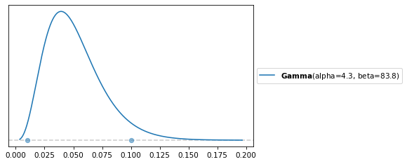
For the standard deviation of efficacy, we also use a gamma distribution, with a high-density interval wide enough to cover all likely values.
dist, plot = pz.maxent(pz.Gamma(), lower=100, upper=120, mass=0.95)
sigma_params = dist.params_dict
sigma_params
{'alpha': 463.6083812559706, 'beta': 4.2172887180676595}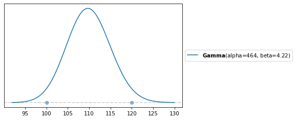
sigma_noise controls the magnitude of the perturbations to the distribution of efficacy.
The following prior is weakly informative,
dist, plot = pz.maxent(pz.Gamma(), lower=0.03, upper=0.3, mass=0.95)
sigma_noise_params = dist.params_dict
sigma_noise_params
{'alpha': 4.30010837792882, 'beta': 27.947108661773417}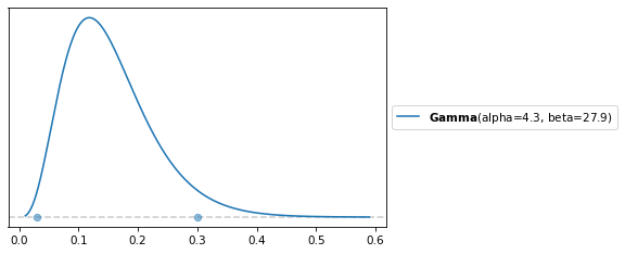
Now here’s the model.
def make_model(N_test, counts_obs):
    with pm.Model() as model:
        # Latent efficacy distribution
        mu = pm.Normal("mu", mu=500, sigma=30)
        sigma = pm.Gamma("sigma", **sigma_params)

        # Prior for the parameter of the selection effect
        beta = pm.Gamma("beta", **beta_params)

        # Compute log PDF of the hypothetical distribution of efficacy
        log_pdf = pm.logp(pm.Normal.dist(mu=mu, sigma=sigma), full_thetas)

        # Generate perturbations in the center region
        sigma_noise = pm.Gamma("sigma_noise", **sigma_noise_params)
        log_noise_raw = pm.ZeroSumNormal("log_noise_raw", sigma=sigma_noise,
                                         shape=(len(thetas),))

        # --- Detrend log_noise ---
        # slope = (x·y) / (x·x)
        x = thetas_scaled
        slope = pm.math.dot(log_noise_raw, x) / pm.math.dot(x, x)
        log_noise = pm.Deterministic("log_noise", log_noise_raw - slope * x)

        # Perturb the distribution
        perturbed_log_pdf = log_pdf[center_mask].inc(log_noise)

        # Normalize and convert to probabilities
        normalizer = pm.math.logsumexp(perturbed_log_pdf)
        pdf = pm.Deterministic("pdf", pm.math.exp(perturbed_log_pdf - normalizer))

        # Roll up the tail probabilities
        left_mass = pdf[left_mask].sum()
        right_mass = pdf[right_mask].sum()
        center_pdf = pdf[center_mask]

        # Add the tail probabilities to the extreme scores
        center_pdf = center_pdf[0].inc(left_mass)
        center_pdf = center_pdf[-1].inc(right_mass)

        # Selection model (linear on logit scale)
        logits = beta * thetas_scaled
        p_take = pm.Deterministic("p_take", pm.math.sigmoid(logits))

        # Test-taker distribution
        test_unnorm = center_pdf * p_take
        test_pdf = test_unnorm / pm.math.sum(test_unnorm)

        # Multinomial likelihood for binned scores
        pm.Multinomial("obs_bins", n=N_test, p=test_pdf, observed=counts_obs)

    return model
We use a ZeroSumNormal so the perturbations can shift mass around but cannot add or remove mass overall.
Then we remove any linear trend in the perturbations to prevent them from absorbing the shape that should be attributed to the selection function.
Here’s a sample from the prior distributions.
model = make_model(N_test, counts_obs)

with model:
    prior = pm.sample_prior_predictive(1000)
Sampling: [beta, log_noise_raw, mu, obs_bins, sigma, sigma_noise]
az.plot_posterior(prior, group='prior', var_names=['sigma']);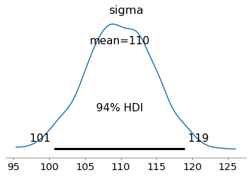
az.plot_posterior(prior, group='prior', var_names=['beta']);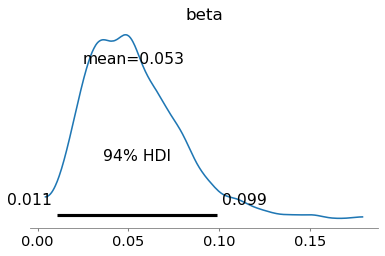
And here’s how we fit the model.
with model:
    idata1 = pm.sample(
        tune=1000,
        draws=2000,
        target_accept=0.95,
        nuts_sampler="nutpie",
        nuts_sampler_kwargs=dict(
            low_rank_modified_mass_matrix=True,
            mass_matrix_eigval_cutoff=3,
            mass_matrix_gamma=1e-5
        )
)The diagnostics are not perfect, but good enough for the current purposes: the posterior predictive check and parameter recovery test.
pm.summary(idata1, var_names=['mu', 'sigma', 'beta', 'sigma_noise'])pm.plot_trace(idata1, var_names=['mu', 'sigma', 'beta'])
decorate()
plt.savefig("figs/selection_bias19.png", dpi=300)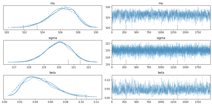
Here are the posterior distributions.
pm.plot_posterior(idata1, var_names=['mu', 'sigma'])
decorate()
plt.savefig("figs/selection_bias20.png", dpi=300)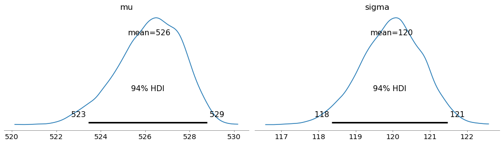
pm.plot_posterior(idata1, var_names=['beta'])
decorate()
plt.savefig("figs/selection_bias21.png", dpi=300)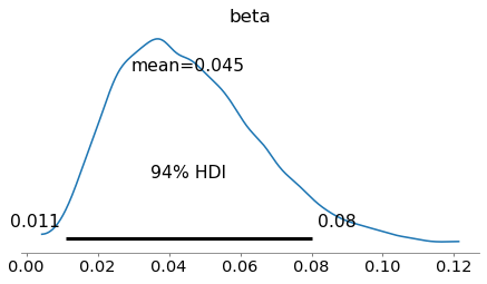
az.plot_forest(idata1, var_names='log_noise', combined=True);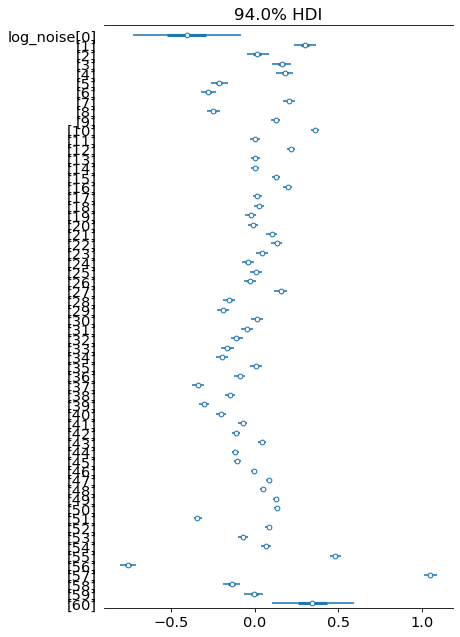
log_noise = np.median(az.extract(idata1)['log_noise'], axis=1)
plt.plot(thetas, log_noise)
decorate(xlabel='Score')
plt.savefig("figs/selection_bias22.png", dpi=300)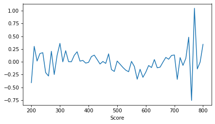
pdf = np.median(az.extract(idata1)['pdf'], axis=1)
plt.plot(full_thetas, pdf)
decorate(xlabel='Score')
plt.savefig("figs/selection_bias23.png", dpi=300)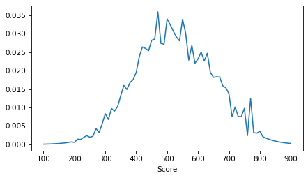
Here’s what the selection function looks like, indicating the relative probability of taking the test for a range of potential scores. These probabilities are scaled so the midpoint is 50%. The left side indicates how much less likely someone is to take the test if their potential score is low.
plot_selection_function(idata1, thetas_scaled)
decorate(xlabel='Score', ylabel='Prob(test)', title='Selection effect')
plt.savefig("figs/selection_bias24.png", dpi=300)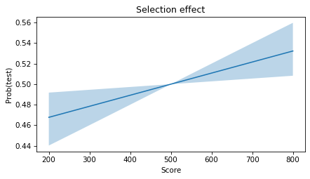
To see how reliable this estimate is, let’s run a parameter recovery test.
Posterior predictive check
with model:
    post_pred = pm.sample_posterior_predictive(idata1)
Sampling: [obs_bins]
obs_bins_post_pred = az.extract(post_pred, group='posterior_predictive')['obs_bins']
obs_bins_post_pred.shape
(61, 8000)medians = np.median(obs_bins_post_pred, axis=-1)
medians.shape(61,)hdi_bounds = az.hdi(post_pred['posterior_predictive']['obs_bins'], hdi_prob=0.94)
low, high = hdi_bounds['obs_bins'].Tcolor_map = {'Male': 'C0', 'Female': 'C1'}
plt.fill_between(
thetas,
low,
high,
color='gray',
alpha=0.3,
)
plt.plot(thetas, medians, color='gray', label=f'{year} {sex} model')
df_map[year][sex].plot(color=color_map[sex], label=f'{year} {sex} data')
decorate(title='Posterior predictive distribution')
plt.savefig("figs/selection_bias25.png", dpi=300)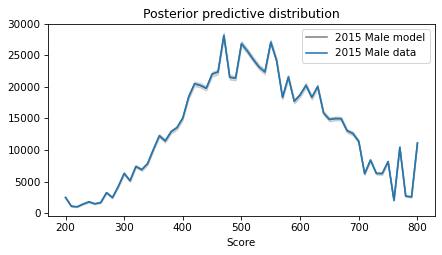
Parameter recovery
We’ll use the following function to generate data given known parameters.
def generate_with_pymc(
    N_test, true_mu, true_sigma, true_beta, true_log_noise, random_seed=123
):
    with pm.Model() as gen:
        # Fixed “true” parameters as constants (no uncertainty)
        mu = pm.Data("mu", true_mu)
        sigma = pm.Data("sigma", true_sigma)
        beta = pm.Data("beta", true_beta)
        log_noise = pm.Data("log_noise", true_log_noise)

        # Compute perturbed log population PDF
        log_pdf = pm.logp(pm.Normal.dist(mu=mu, sigma=sigma), full_thetas)
        perturbed_log_pdf = log_pdf[center_mask].inc(log_noise)

        normalizer = pm.math.logsumexp(perturbed_log_pdf)
        pdf = pm.Deterministic("pdf", pm.math.exp(perturbed_log_pdf - normalizer))

        # tails → center
        left_mass  = pdf[left_mask].sum()
        right_mass = pdf[right_mask].sum()
        center_pdf = pdf[center_mask]
        center_pdf = center_pdf[0].inc(left_mass)
        center_pdf = center_pdf[-1].inc(right_mass)

        # selection
        logits = beta * thetas_scaled
        p_take = pm.Deterministic("p_take", pm.math.sigmoid(logits))

        # test-taker score distribution
        test_unnorm = center_pdf * p_take
        test_pdf = pm.Deterministic("test_pdf", test_unnorm / test_unnorm.sum())

        # generate synthetic data
        obs_bins = pm.Multinomial("obs_bins", n=N_test, p=test_pdf)

        prior_pred = pm.sample_prior_predictive(
            draws=1,
            var_names=["obs_bins", "test_pdf", "p_take", "pdf"],
            random_seed=random_seed,
        )
        return prior_pred
As an example, we’ll test it with parameters based on the previous example.
N_test = 800_000
true_mu = 510
true_sigma = 110
true_beta = 0.03
true_log_noise = log_noise

prior_pred = generate_with_pymc(
    N_test, true_mu, true_sigma, true_beta, true_log_noise, random_seed=4
)
Sampling: [obs_bins]
counts_draw = prior_pred.prior["obs_bins"].values.squeeze()
counts_draw
array([ 1994, 1008, 877, 1371, 1719, 1464, 1691, 3247, 2528,
4434, 6754, 5600, 7998, 7722, 8718, 11482, 14182, 13467,
15109, 15871, 18048, 21667, 24307, 23823, 23111, 25708, 26144,
32311, 24941, 24441, 30497, 28573, 26949, 25047, 23842, 28191,
25056, 18696, 21282, 17346, 17731, 18486, 16857, 17627, 13541,
12452, 11780, 11601, 9814, 9366, 8111, 4134, 5371, 3926,
3686, 4755, 1069, 5569, 1274, 1241, 4393])And we can confirm that the generated data resembles the actual data it is based on.
pmf = Pmf(counts_draw, thetas)
pmf.normalize()
pmf.plot(label='draw')

pmf = Pmf(counts_obs, thetas)
pmf.normalize()
pmf.plot(label='observed')

print(pmf.mean())
decorate()
plt.savefig("figs/selection_bias26.png", dpi=300)
527.1939174788187
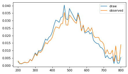
Now let’s run the model on the generated data.
model = make_model(N_test, counts_draw)with model:
idata2 = pm.sample(
tune=1000,
draws=2000,
target_accept=0.95,
nuts_sampler="nutpie",
nuts_sampler_kwargs=dict(
low_rank_modified_mass_matrix=True,
mass_matrix_eigval_cutoff=3,
mass_matrix_gamma=1e-5
)
)The diagnostics are good enough -- although some of the effective sample sizes are small.
pm.summary(idata2, var_names=['mu', 'sigma', 'beta', 'sigma_noise'])Ideally, the true values should fall within the posterior HDIs.
The estimate of mu is a little low, but the HDI covers the true value.
def plot_posterior(trace, var_name, x_true):
    # Extract posterior samples
    samples = az.extract(trace)[var_name].to_numpy()
    mean = samples.mean()

    # Plot the KDE and get axis
    ax = az.plot_posterior(trace, var_names=var_name, hdi_prob='hide')

    # Get the height of the axis
    ymin, ymax = ax.get_ylim()

    # Plot vertical lines at true value and mean
    plt.vlines(mean, 0, ymax * 0.85, ls=':', color='gray')
    plt.vlines(x_true, 0, ymax * 0.5, ls='-', color='orange')
    plt.text(x_true, ymax * 0.5, f'actual={x_true}', ha='center', fontsize=14)
    decorate()
plot_posterior(idata2, 'mu', true_mu)
plt.savefig("figs/selection_bias30.png", dpi=300)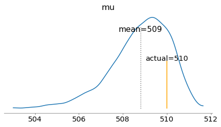
The estimate of sigma is a little high.
plot_posterior(idata2, 'sigma', true_sigma)
plt.savefig("figs/selection_bias31.png", dpi=300)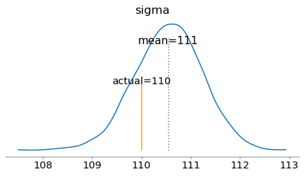
And the estimate of beta is a little high, but the HDI covers the true value.
plot_posterior(idata2, 'beta', true_beta)
plt.savefig("figs/selection_bias32.png", dpi=300)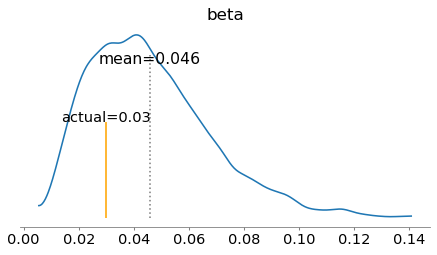
The parameter recovery test is pretty good.
But with data from only a single year, we can’t be confident in the estimates, in part because the selection parameter and the perturbations compete to explain the shape of the distribution. That’s why we need a hierarchical model.
Hierarchical
A hierarchical model makes it possible to share information between years and sexes. In particular, recall that the distribution of scores appears to be different between sexes but consistent from year to year. And the perturbations in the distribution of scores appear to be different from year to year but consistent between sexes. The hierarchical model can take advantage of these consistencies.
We’ll keep the parameters of the selection model unpooled, so we estimate values separately for each combination of year and sex.
First let’s get the data into shape for the hierarchical model.
def get_counts_obs(year, sex):
    return df_map[year].loc[thetas, sex]
years = [2011, 2012, 2013, 2014, 2015]
sexes = ['Male', 'Female']
count_array = np.array([
[get_counts_obs(year, sex=sex) for sex in sexes]
for year in years
])
count_array.shape # (n_years, n_sexes, n_scores)(5, 2, 61)N_test_array = count_array.sum(axis=2)
N_test_arrayarray([[770605, 876518],
[778142, 886337],
[776092, 883955],
[783570, 888825],
[794802, 903719]])We’ll define coordinates for the various dimensions, which makes the model easier to read and validate.
coords = {
    'year': years,
    'sex': sexes,
    'full_score': full_thetas,    # 81
    'score': thetas,     # 61
}
Here’s the hierarchical model.
with pm.Model(coords=coords) as model:
    # Data
    counts_pt = pm.Data("counts", count_array, dims=("year", "sex", "score"))
    N_test_pt = pm.Data("N_test", N_test_array, dims=("year", "sex"))

    # Population distribution parameters per sex
    mu = pm.Normal("mu", mu=500, sigma=30, dims="sex")
    sigma = pm.Gamma("sigma", **sigma_params, dims="sex")

    # Parameters of the selection functions
    beta = pm.Gamma("beta", **beta_params, dims=["year", "sex"])
    #beta = pm.HalfNormal("beta", 0.2, dims=["year", "sex"])

    # Base log-probability from the Normal distribution (sex, full_score)
    log_pdf = pm.logp(pm.Normal.dist(mu=mu[:, None],
                                     sigma=sigma[:, None]),
                                     full_thetas[None, :])

    # Generate noise
    sigma_noise = pm.Gamma("sigma_noise", **sigma_noise_params)
    log_noise_raw = pm.ZeroSumNormal("log_noise_raw", sigma=sigma_noise,
                                     dims=["year", "score"])

    # --- Detrend log_noise along the score axis (per year) ---
    x = thetas_scaled                        # shape: (score,)
    x2_sum = pm.math.sum(x * x)              # scalar
    slope = pm.math.sum(log_noise_raw * x[None, :], axis=-1) / x2_sum   # shape: (year,)
    log_noise = pm.Deterministic(
        "log_noise",
        log_noise_raw - slope[:, None] * x[None, :]
    )

    zeros = pt.zeros((len(years), len(full_thetas)))
    log_noise_full = zeros[:, center_mask].inc(log_noise)

    # Add noise to log_pdf, broadcast to (year, sex, full_score)
    perturbed_log_pdf = log_pdf[None, :, :] + log_noise_full[:, None, :]

    # Convert to probabilities (year, sex, full_score)
    normalizer = pm.math.logsumexp(perturbed_log_pdf, axis=-1, keepdims=True)
    pdf = pm.Deterministic("pdf", pm.math.exp(perturbed_log_pdf - normalizer))

    # Compute center_pdf and add tail masses
    left_mass = pdf[:, :, left_mask].sum(axis=-1)    # (year, sex)
    right_mass = pdf[:, :, right_mask].sum(axis=-1)  # (year, sex)
    center_pdf = pdf[:, :, center_mask]              # (year, sex, score)

    center_pdf = center_pdf[:, :, 0].inc(left_mass)
    center_pdf = center_pdf[:, :, -1].inc(right_mass)

    # Selection model
    logits = beta[:, :, None] * thetas_scaled[None, None, :]  # (year, sex, score)
    p_take = pm.Deterministic("p_take", pm.math.sigmoid(logits))

    # Test-taker distribution
    test_unnorm = center_pdf * p_take
    test_pdf = pm.Deterministic("test_pdf", test_unnorm / test_unnorm.sum(axis=-1, keepdims=True))

    # Multinomial likelihood for score bins
    pm.Multinomial("obs_bins", n=N_test_pt, p=test_pdf, observed=counts_pt,
                   dims=["year", "sex", "score"])
with model:
idata3 = pm.sample(
tune=1000,
draws=1000,
target_accept=0.90,
nuts_sampler="nutpie",
nuts_sampler_kwargs=dict(
low_rank_modified_mass_matrix=True,
mass_matrix_eigval_cutoff=3,
mass_matrix_gamma=1e-5
)
)We’ll save the trace so we can run additional analysis later without running the model again.
# idata3.to_netcdf("selection_bias3_idata.nc")The diagnostics are good -- r_hats are 1.0 across the board, and the effective sample sizes are sufficient.
pm.summary(idata3, var_names=['mu', 'sigma', 'beta', 'sigma_noise'])pm.plot_trace(idata3, var_names=['mu', 'sigma', 'beta', 'sigma_noise'])
decorate()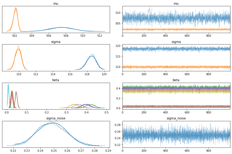
az.plot_forest(idata3, var_names='log_noise', combined=True);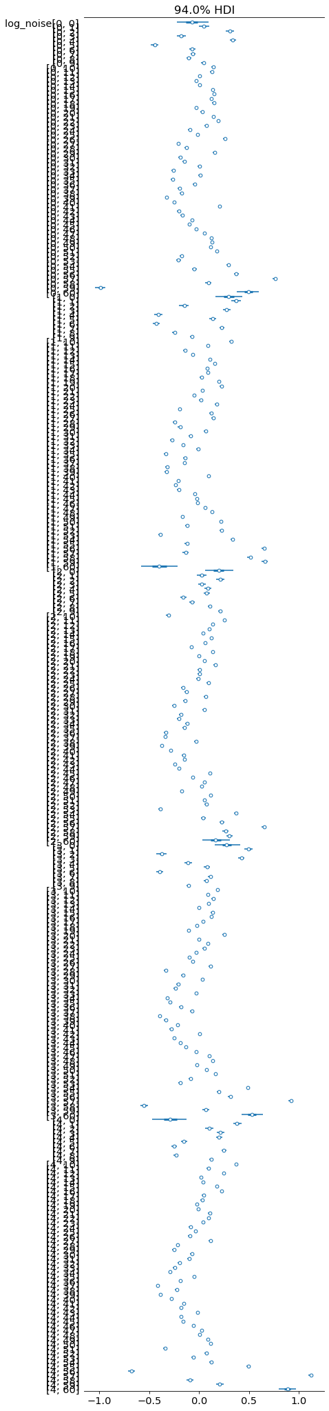
Here are the posterior distributions.
def plot_two_posteriors(idata, varname):
    ax = plt.gca()
    az.plot_posterior(idata.posterior[varname].sel(sex="Male"),
                      ax=ax, hdi_prob='hide', color="C0", label="Male")
    az.plot_posterior(idata.posterior[varname].sel(sex="Female"),
                      ax=ax, hdi_prob='hide', color="C1", label="Female")
    decorate()
plot_two_posteriors(idata3, "mu")
plt.savefig("figs/selection_bias33.png", dpi=300)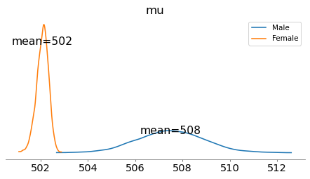
The posterior means of the mu parameters are substantially closer together than the 31-34 point difference seen in the mean test scores.
plot_two_posteriors(idata3, "sigma")
plt.savefig("figs/selection_bias34.png", dpi=300)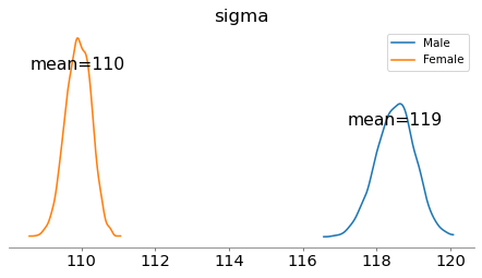
The estimated standard deviation is considerably higher for males.
pm.plot_posterior(idata3, var_names=['beta'])
decorate()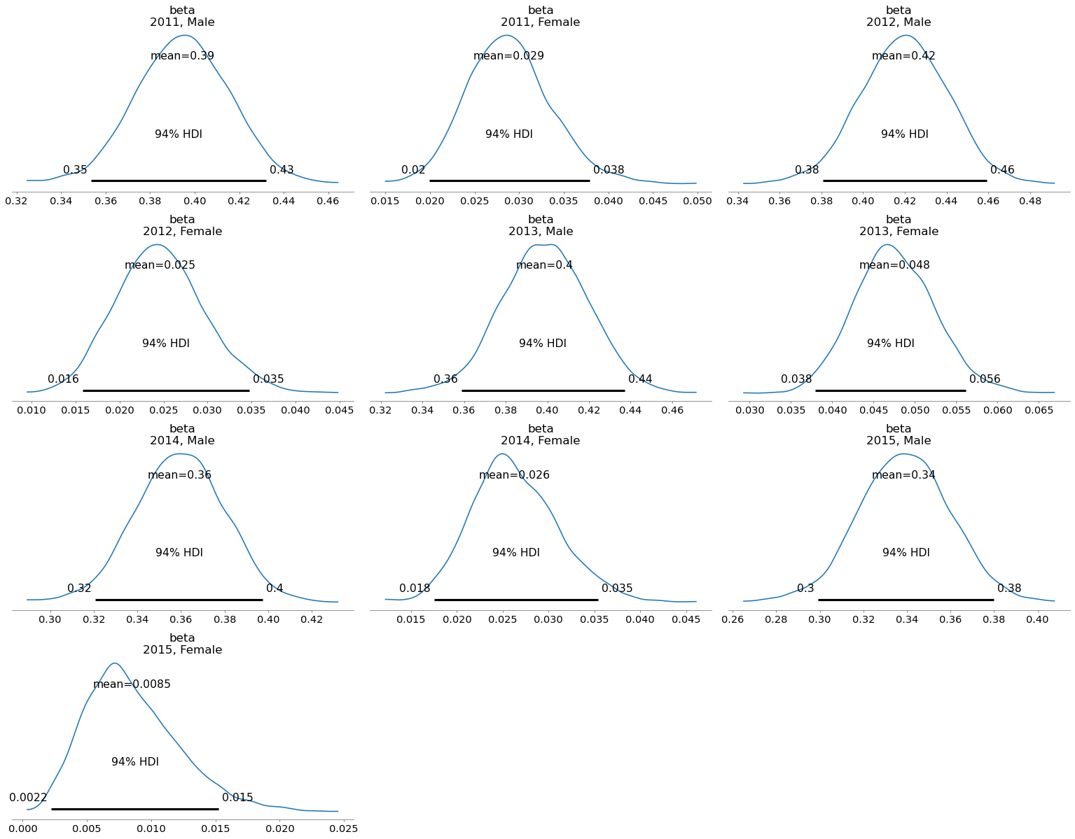
Here are the estimated selection functions for male test-takers. They are consistent from year to year, and show a strong selection effect.
for year in years:
    idata_one = idata3.sel(year=year, sex="Male")
    plot_selection_function(idata_one, thetas_scaled)

ylim = [0.2, 0.8]
decorate(xlabel='Latent efficacy', ylabel='Prob(taking test)',
         title='Male 2011-2015', ylim=ylim)
plt.savefig("figs/selection_bias38.png", dpi=300)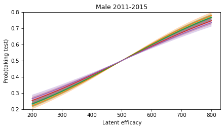
Here are the estimated selection functions for female test-takers. They are reasonably consistent from year to year, and show a much weaker selection effect.
for year in years:
    idata_one = idata3.sel(year=year, sex="Female")
    plot_selection_function(idata_one, thetas_scaled)

decorate(xlabel='Latent efficacy', ylabel='Prob(taking test)',
         title='Female 2011-2015', ylim=ylim)
plt.savefig("figs/selection_bias39.png", dpi=300)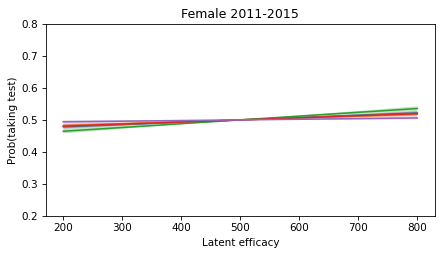
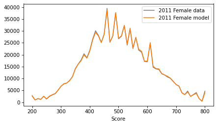
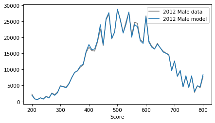
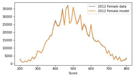
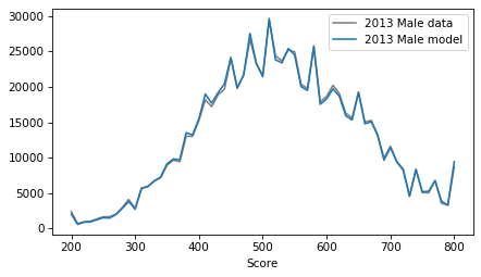
If we generate a sample from the posterior predictive distribution, we can confirm that the score distributions are similar to the observed data.
with model:
    post_pred = pm.sample_posterior_predictive(idata3)
Sampling: [obs_bins]
obs_bins_post_pred = az.extract(post_pred, group='posterior_predictive')['obs_bins']
obs_bins_post_pred.shape
(5, 2, 61, 4000)medians = np.median(obs_bins_post_pred, axis=-1)
medians.shape(5, 2, 61)for i, year in enumerate(years):
for j, sex in enumerate(sexes):
plt.figure()
df_map[year][sex].plot(color='gray', label=f'{year} {sex} data')
plt.plot(thetas, medians[i, j], color=color_map[sex], label=f'{year} {sex} model')
decorate()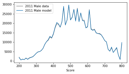
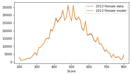
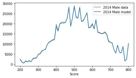
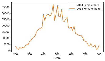
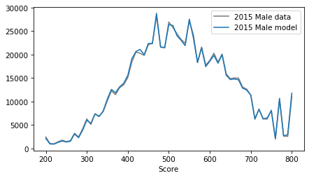
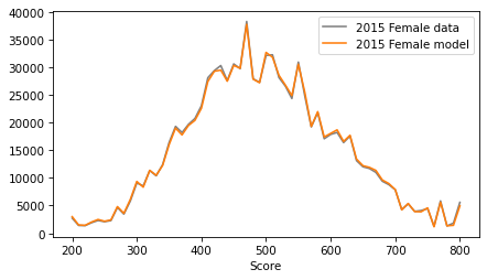
fig, axes = plt.subplots(nrows=2, ncols=5, figsize=(18, 6), sharex=True, sharey=True)

for i, year in enumerate(years):
    for j, sex in enumerate(sexes):
        ax = axes[j, i]   # row = sex index, col = year index

        df_map[year][sex].plot(ax=ax, color='gray', label=f'{year} {sex} data')
        ax.plot(thetas, medians[i, j], color=color_map[sex], label=f'{year} {sex} model')

        plt.sca(ax)
        decorate(title=f'{year} {sex}', legend=False)

plt.tight_layout(rect=[0, 0, 1, 0.95])
plt.savefig("figs/selection_bias40.png", dpi=300)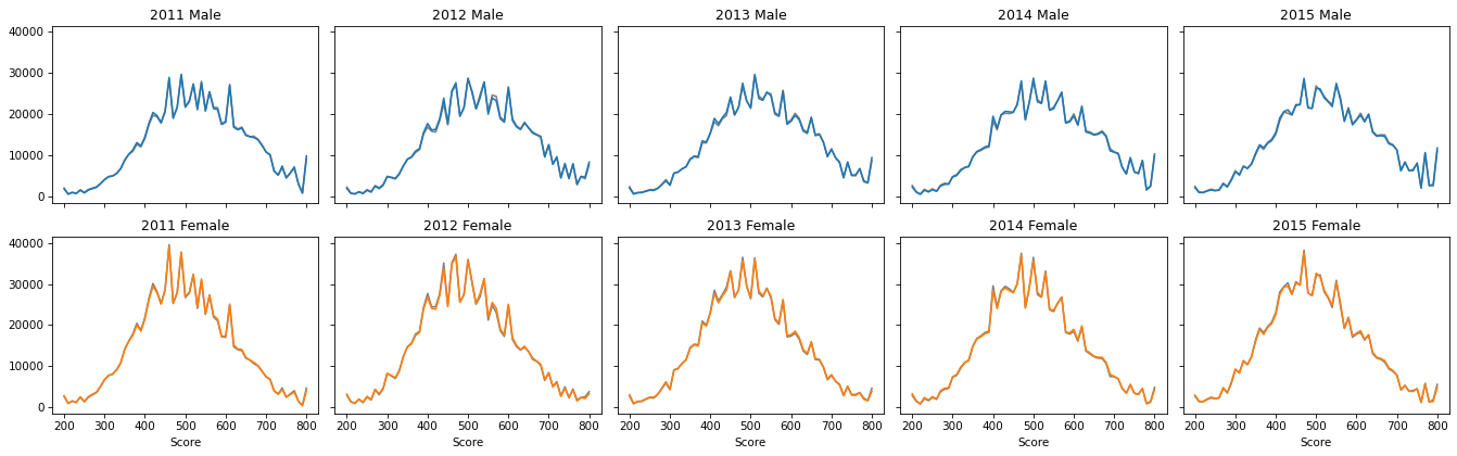
These results depend strongly on the assumption that the latent distribution of efficacy is Gaussian -- if the distribution of scores is skewed, that is taken to imply a selection effect. We can’t rule out the possibility that the underlying distribution is truly skewed.
The results are also sensitive to a free parameter of the model, the amount of deviation from a normal distribution that can be attributed to the quirks of SAT scoring. We have set this parameter to the lowest value that allows the model to reproduce the quirks without obscuring the effects we are interested in: selection bias and differences in the latent distributions for males and females.
So we should probably not take the estimated selection functions too seriously. For example, the selection functions for males suggest that someone with the efficacy to score 800 is 2-3 times more likely to take the SAT than someone whose expected score is 200. It’s hard to say whether that’s realistic.
However, the results of the hierarchical model provide strong evidence that:
The selection effect is substantially stronger for males than females, and
The difference in selection effects could explain a large part of the observed difference in scores between male and female test-takers.
While the difference in scores is consistently 31-34 points, the difference in average efficacy might be only 8 points.