Predicting Crime#
This is the first in a series of notebooks that make up a case study on classification and algorithmic fairness. This case study is part of the Elements of Data Science curriculum. Click here to run this notebook on Colab.
This chapter and the next make up a case study related to “Machine Bias”, an article published by ProPublica in 2016. The article explores the use of predictive algorithms in the criminal justice system.
In this chapter, we’ll replicate the analysis described in the article and compute statistics that evaluate these algorithms, including accuracy, predictive value, end error rates.
In the next chapter, we’ll review arguments presented in a response article published in the Washington Post. We’ll compute and interpret calibration curves, and explore the trade-offs between predictive value and error rates.
In an additional notebook (not in the book), I apply the same analysis to evaluate the performance of classification for male and female defendants.
You can read the ProPublica article at https://www.propublica.org/article/machine-bias-risk-assessments-in-criminal-sentencing.
from os.path import basename, exists

def download(url):
    filename = basename(url)
    if not exists(filename):
        from urllib.request import urlretrieve

        local, _ = urlretrieve(url, filename)
        print("Downloaded " + local)

download(
    "https://raw.githubusercontent.com/AllenDowney/RecidivismCaseStudy/v1/rcs_utils.py"
)

from rcs_utils import values
Machine Bias#
We’ll start by replicating the analysis reported in “Machine Bias”, by Julia Angwin, Jeff Larson, Surya Mattu and Lauren Kirchner, and published by ProPublica in May 2016.
This article is about a statistical tool called COMPAS which is used in some criminal justice systems to inform decisions about which defendants should be released on bail before trial, how long convicted defendants should be imprisoned, and whether prisoners should be released on parole. COMPAS uses information about defendants to generate a “risk score” which is intended to quantify the risk that the defendant would commit another crime if released.
Read more about COMPAS at https://en.wikipedia.org/wiki/COMPAS_(software).
See the ProPublica analysis of the data at https://github.com/propublica/compas-analysis/blob/master/Compas Analysis.ipynb.
The authors of the ProPublica article used public data to assess the accuracy of those risk scores. They explain:
We obtained the risk scores assigned to more than 7,000 people arrested in Broward County, Florida, in 2013 and 2014 and checked to see how many were charged with new crimes over the next two years, the same benchmark used by the creators of the algorithm.
In the notebook that contains their analysis, they explain in more detail:
We filtered the underlying data from Broward county to include only those rows representing people who had either recidivated in two years, or had at least two years outside of a correctional facility.
[…] Next, we sought to determine if a person had been charged with a new crime subsequent to the crime for which they were COMPAS screened. We did not count traffic tickets and some municipal ordinance violations as recidivism. We did not count as recidivists people who were arrested for failing to appear at their court hearings, or people who were later charged with a crime that occurred prior to their COMPAS screening.
If you are not familiar with the word “recidivism”, it usually means a tendency to relapse into criminal behavior. In this context, a person is a “recidivist” if they are charged with another crime within two years of release. However, note that there is a big difference between committing another crime and being charged with another crime. We will come back to this issue.
The authors of the ProPublica article use this data to evaluate how well COMPAS predicts the risk that a defendant will be charged with another crime within two years of their release. Among their findings, they report:
[…] the algorithm was somewhat more accurate than a coin flip. Of those deemed likely to re-offend, 61 percent were arrested for any subsequent crimes within two years.
[…] In forecasting who would re-offend, the algorithm made mistakes with Black and White defendants at roughly the same rate but in very different ways.
The formula was particularly likely to falsely flag Black defendants as future criminals, wrongly labeling them this way at almost twice the rate as White defendants.
White defendants were mislabeled as low risk more often than Black defendants.
This discrepancy suggests that the use of COMPAS in the criminal justice system is racially biased.
Since the ProPublica article was published, it has been widely discussed in the media, and a number of researchers have published responses. In order to evaluate the original article and the responses it provoked, there are some technical issues you need to understand. The goal of this case study is to help you analyze the arguments and interpret the statistics they are based on.
Replicating the Analysis#
The data used in “Machine Bias” is available from ProPublica. Instructions for downloading it are in the notebook for this chapter.
We can use Pandas to read the file and make a DataFrame.
import pandas as pd

cp = pd.read_csv("compas-scores-two-years.csv")
cp.shape
(7214, 53)
The dataset includes one row for each defendant, and 53 columns, including risk scores computed by COMPAS and demographic information like age, sex, and race.
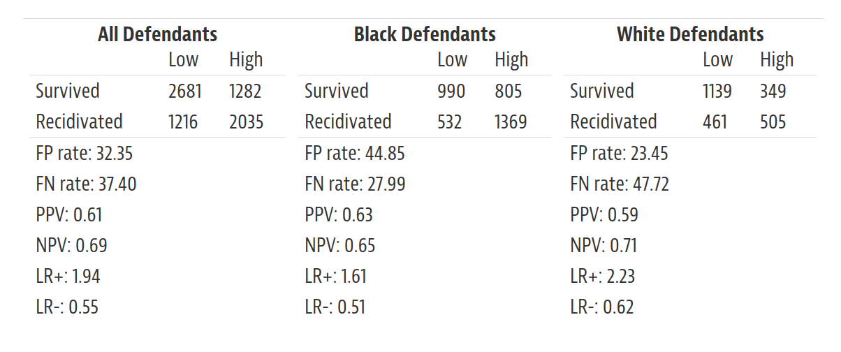
The authors of “Machine Bias” describe their analysis in a supplemental article called “How We Analyzed the COMPAS Recidivism Algorithm”. It includes this table, which summarizes many of the results they report:
The supplemental article is available from https://www.propublica.org/article/how-we-analyzed-the-compas-recidivism-algorithm.
The table summarizes results for all defendants and two subgroups: defendants classified as White (“Caucasian” in the original dataset) and Black (“African-American”). For each group, the summary includes several metrics, including:
FP rate: false positive rate
FN rate: false negative rate
PPV: positive predictive value
NPV: negative predictive value
LR+: positive likelihood ratio
LR-: negative likelihood ratio
I will explain what these metrics mean and how to compute them, and we’ll replicate the results in this table. But first let’s examine and clean the data.
Here are the values of decile_score, which is the output of the COMPAS algorithm.
1 is the lowest risk category; 10 is the highest.
values(cp["decile_score"])
decile_score
1     1440
2      941
3      747
4      769
5      681
6      641
7      592
8      512
9      508
10     383
Name: count, dtype: int64
It’s important to note that COMPAS is not a binary classifier – that is, it does not predict that a defendant will or will not recidivate. Rather, it gives each defendant a score that is intended to reflect the risk that they will recidivate.
In order to evaluate the performance of COMPAS, the authors of the ProPublica article chose a threshold, 4, and defined decile scores at or below the threshold to be “low risk”, and scores above the threshold to be “high risk”.
Their choice of the threshold is arbitrary.
Later, we’ll see what happens with other choices, but we’ll start by replicating the original analysis.
We’ll create a Boolean Series called high_risk that’s True for respondents with a decile score greater than 4.
high_risk = cp["decile_score"] > 4
high_risk.name = "HighRisk"
values(high_risk)
HighRisk
False    3897
True     3317
Name: count, dtype: int64
The column two_year_recid indicates whether a defendant was charged with another crime during a two year period after the original charge when they were not in a correctional facility.
values(cp["two_year_recid"])
two_year_recid
0    3963
1    3251
Name: count, dtype: int64
Let’s create another Series, called new_charge, that is True for defendants who were charged with another crime within two years.
new_charge = cp["two_year_recid"] == 1
new_charge.name = "NewCharge"
values(new_charge)
NewCharge
False    3963
True     3251
Name: count, dtype: int64
If we make a cross-tabulation of new_charge and high_risk, the result is a DataFrame that indicates how many defendants are in each of four groups:
pd.crosstab(new_charge, high_risk)
| HighRisk | False | True |
|---|---|---|
| NewCharge | ||
| False | 2681 | 1282 |
| True | 1216 | 2035 |
This table is called a confusion matrix or error matrix. Reading from left to right and top to bottom, the elements of the matrix show the number of respondents who were:
Classified as low risk and not charged with a new crime: there were 2681 true negatives – that is, cases where the test was negative (not high risk) and the prediction turned out to be correct (no new charge).
High risk and not charged: there were 1282 false positives – that is, cases where the test was positive and the prediction was incorrect.
Low risk and charged: there were 1216 false negatives – that is, cases where the test was negative (low risk) and the prediction was incorrect (the defendant was charged with a new crime).
High risk and charged: there were 2035 true positives – that is, cases where the test was positive and the prediction was correct.
The values in this matrix are consistent with the values in the ProPublica article, so we can confirm that we are replicating their analysis correctly.
Now let’s check the confusion matrices for White and Black defendants.
Here are the values of race:
values(cp["race"])
race
African-American    3696
Asian                 32
Caucasian           2454
Hispanic             637
Native American       18
Other                377
Name: count, dtype: int64
Here’s a Boolean Series that’s true for White defendants.
white = cp["race"] == "Caucasian"
white.name = "white"
values(white)
white
False    4760
True     2454
Name: count, dtype: int64
And here’s the confusion matrix for White defendants.
pd.crosstab(new_charge[white], high_risk[white])
| HighRisk | False | True |
|---|---|---|
| NewCharge | ||
| False | 1139 | 349 |
| True | 461 | 505 |
black is a Boolean Series that is True for Black defendants.
black = cp["race"] == "African-American"
black.name = "black"
values(black)
black
False    3518
True     3696
Name: count, dtype: int64
And here’s the confusion matrix for Black defendants.
pd.crosstab(new_charge[black], high_risk[black])
| HighRisk | False | True |
|---|---|---|
| NewCharge | ||
| False | 990 | 805 |
| True | 532 | 1369 |
All of these results are consistent with the ProPublica article. However, before we go on, I want to address an important issue with this dataset: data bias.
Data Bias#
Systems like COMPAS are trying to predict whether a defendant will commit another crime if released. But the dataset reports whether a defendant was charged with another crime. Not everyone who commits a crime gets charged (not even close). The probability of getting charged for a particular crime depends on the type of crime and location; the presence of witnesses and their willingness to work with police; the decisions of police about where to patrol, what crimes to investigate, and who to arrest; and decisions of prosecutors about who to charge.
It is likely that every one of these factors depends on the race of the defendant. In this dataset, the prevalence of new charges is higher for Black defendants, but that doesn’t necessarily mean that the prevalence of new crimes is higher. If the dataset is affected by racial bias in the probability of being charged, prediction algorithms like COMPAS will be biased, too. In discussions of whether and how these systems should be used in the criminal justice system, this is an important issue.
However, I am going to put it aside for now in order to focus on understanding the arguments posed in the ProPublica article and the metrics they are based on. For the rest of this chapter I will take the “recidivism rates” in the dataset at face value – but I will try to be clear about what they mean and don’t mean.
Arranging the confusion matrix#
In the previous section I arranged the confusion matrix to be consistent with the ProPublica article, to make it easy to check for consistency. But it is more common to arrange the matrix like this:
Predicted positive |
Predicted negative |
|
|---|---|---|
Actual positive |
True positive (TP) |
False negative (FN) |
Actual negative |
False positive (FP) |
True negative (TN) |
In this arrangement:
The actual conditions are down the rows.
The predictions are across the columns.
The rows and columns are sorted so true positives are in the upper left and true negatives are in the lower right.
In the context of the ProPublica article:
“Predicted positive” means the defendant is classified as high risk.
“Predicted negative” means low risk.
“Actual positive” means the defendant was charged with a new crime.
“Actual negative” means they were not charged with a new crime during the follow-up period.
The following function makes a confusion matrix with this arrangement:
import numpy as np


def make_matrix(cp, threshold=4):
    """Make a confusion matrix.

    cp: DataFrame
    threshold: default is 4

    returns: DataFrame containing the confusion matrix
    """
    a = np.where(cp["decile_score"] > threshold, "Pred Positive", "Pred Negative")
    high_risk = pd.Series(a, name="")

    a = np.where(cp["two_year_recid"] == 1, "Positive", "Negative")
    new_charge = pd.Series(a, name="Actual")

    matrix = pd.crosstab(new_charge, high_risk)
    matrix.sort_index(axis=0, ascending=False, inplace=True)
    matrix.sort_index(axis=1, ascending=False, inplace=True)

    return matrix
Going forward, we’ll present confusion matrices in this format.
For example, here is the confusion matrix for all defendants.
matrix_all = make_matrix(cp)
matrix_all
| Pred Positive | Pred Negative | |
|---|---|---|
| Actual | ||
| Positive | 2035 | 1216 |
| Negative | 1282 | 2681 |
Accuracy#
Based on these results, how accurate is COMPAS as a binary classifier? Well, it turns out that there are a lot of ways to answer that question. One of the simplest is overall accuracy, which is the fraction (or percentage) of correct predictions. To compute accuracy, it is convenient to extract from the confusion matrix the number of true positives, false negatives, false positives, and true negatives.
tp, fn, fp, tn = matrix_all.to_numpy().flatten()
The number of true predictions is tp + tn.
The number of false predictions is fp + fn.
So we can compute the fraction of true predictions like this:
def percent(x, y):
    """Compute the percentage `x/(x+y)*100`."""
    return x / (x + y) * 100
accuracy = percent(tp + tn, fp + fn)
accuracy
65.37288605489326
As a way to evaluate a binary classifier, accuracy does not distinguish between true positives and true negatives, or false positives and false negatives. But it is often important to make these distinctions, because the benefits of true predictions and true negatives might be different, and the costs of false positives and false negatives might be different.
Predictive Value#
One way to make these distinctions is to compute the “predictive value” of positive and negative tests:
Positive predictive value (PPV) is the fraction of positive tests that are correct.
Negative predictive value (NPV) is the fraction of negative tests that are correct.
In this example, PPV is the fraction of high risk defendants who were charged with a new crime. NPV is the fraction of low risk defendants who “survived” a two year period without being charged.
The following function takes a confusion matrix and computes these metrics.
def predictive_value(m):
    """Compute positive and negative predictive value.

    m: confusion matrix
    """
    tp, fn, fp, tn = m.to_numpy().flatten()
    ppv = percent(tp, fp)
    npv = percent(tn, fn)
    return ppv, npv
Here are the predictive values for all defendants.
ppv, npv = predictive_value(matrix_all)
ppv, npv
(61.350618028338864, 68.79651013600206)
Among all defendants, a positive test is correct about 61% of the time; a negative test result is correct about 69% of the time.
Sensitivity and Specificity#
Another way to characterize the accuracy of a test is to compute
Sensitivity, which is the probability of predicting correctly when the condition is present, and
Specificity, which is the probability of predicting correctly when the condition is absent.
A test is “sensitive” if it detects the positive condition. In this example, sensitivity is the fraction of recidivists who were correctly classified as high risk.
A test is “specific” if it identifies the negative condition. In this example, specificity is the fraction of non-recidivists who were correctly classified as low risk.
The following function takes a confusion matrix and computes sensitivity and specificity.
def sens_spec(m):
    """Compute sensitivity and specificity.

    m: confusion matrix
    """
    tp, fn, fp, tn = m.to_numpy().flatten()
    sens = percent(tp, fn)
    spec = percent(tn, fp)
    return sens, spec
Here are sensitivity and specificity for all defendants.
sens, spec = sens_spec(matrix_all)
sens, spec
(62.59612426945556, 67.65076961897553)
If we evaluate COMPAS as a binary classifier:
About 63% of the recidivists were classified as high risk.
About 68% of the non-recidivists were classified as low risk.
It can be hard to keep all of these metrics straight, especially when you are learning about them for the first time. The following table might help:
Metric |
Definition |
|---|---|
PPV |
TP / (TP + FP) |
Sensitivity |
TP / (TP + FN) |
NPV |
TN / (TN + FN) |
Specificity |
TN / (TN + FP) |
PPV and sensitivity are similar in the sense that they both have true positives in the numerator. The difference is the denominator:
PPV is the ratio of true positives to all positive tests. So it answers the question, “Of all positive tests, how many are correct?”
Sensitivity is the ratio of true positives to all positive conditions. So it answers the question “Of all positive conditions, how many are detected?”
Similarly, NPV and sensitivity both have true negatives in the numerator, but:
NPV is the ratio of true negatives to all negative tests. It answers, “Of all negative tests, how many are correct?”
Specificity is the ratio of true negatives to all negative conditions. It answers, “Of all negative conditions, how many are classified correctly?”
False Positive and Negative Rates#
The ProPublica article reports PPV and NPV, but instead of sensitivity and specificity, it reports their complements:
False positive rate, which is the ratio of false positives to all negative conditions. It answers, “Of all negative conditions, how many are misclassified?”
False negative rate, which is the ratio of false negatives to all positive conditions. It answers, “Of all positive conditions, how many are misclassified?”
In this example:
The false positive rate is the fraction of non-recidivists who were classified as high risk.
The false negative rate is the fraction of recidivists who were classified as low risk.
The following function takes a confusion matrix and computes false positive and false negative rates.
def error_rates(m):
    """Compute false positive and false negative rate.

    m: confusion matrix
    """
    tp, fn, fp, tn = m.to_numpy().flatten()
    fpr = percent(fp, tn)
    fnr = percent(fn, tp)
    return fpr, fnr
Here are the error rates for all defendants.
fpr, fnr = error_rates(matrix_all)
fpr, fnr
(32.349230381024476, 37.40387573054445)
FPR is the complement of specificity, which means they have to add up to 100%
fpr + spec
100.0
And FNR is the complement of sensitivity.
fnr + sens
100.0
So FPR and FNR are just another way of reporting sensitivity and specificity. In general, I prefer sensitivity and specificity over FPN and FNR because
I think the positive framing is easier to interpret than the negative framing, and
I find it easier to remember what “sensitivity” and “specificity” mean.
I find “false positive rate” and “false negative rate” harder to remember. For example, “false positive rate” could just as easily mean either
The fraction of positive tests that are incorrect, or
The fraction of negative conditions that are misclassified.
It is only a convention that the first is called the “false discovery rate” and the second is called “false positive rate”. I suspect I am not the only one that gets them confused.
So, here’s my recommendation: if you have the choice, generally use PPV, NPV, sensitivity and specificity, and avoid the other metrics. However, since the ProPublica article uses FPR and FNR, I will too. They also report LR+ and LR-, but those are combinations of other metrics and not relevant to the current discussion, so we will ignore them.
However, there is one other metric that I think is relevant and not included in the ProPublica tables: prevalence, which is the fraction of all cases where the condition is positive. In the example, it’s the fraction of defendants who recidivate. The following function computes prevalence:
def prevalence(m):
    """Compute prevalence.

    m: confusion matrix
    """
    tp, fn, fp, tn = m.to_numpy().flatten()
    prevalence = percent(tp + fn, tn + fp)
    return prevalence
Here’s the prevalence for all defendants:
prev = prevalence(matrix_all)
prev
45.06515109509287
About 45% of the defendants in this dataset were charged with another crime within two years of their release.
All Metrics#
The following function takes a confusion matrix, computes all the metrics, and puts them in a DataFrame.
def compute_metrics(m, name=""):
    """Compute all metrics.

    m: confusion matrix

    returns: DataFrame
    """
    fpr, fnr = error_rates(m)
    ppv, npv = predictive_value(m)
    prev = prevalence(m)

    index = ["FP rate", "FN rate", "PPV", "NPV", "Prevalence"]
    df = pd.DataFrame(index=index, columns=["Percent"])
    df.Percent = fpr, fnr, ppv, npv, prev
    df.index.name = name
    return df.round(1)
Here are the metrics for all defendants.
compute_metrics(matrix_all, "All defendants")
| Percent | |
|---|---|
| All defendants | |
| FP rate | 32.3 |
| FN rate | 37.4 |
| PPV | 61.4 |
| NPV | 68.8 |
| Prevalence | 45.1 |
Comparing these results to the table from ProPublica, it looks like our analysis agrees with theirs.

Here are the same metrics for Black defendants.
compute_metrics(matrix_black, "Black defendants")
| Percent | |
|---|---|
| Black defendants | |
| FP rate | 44.8 |
| FN rate | 28.0 |
| PPV | 63.0 |
| NPV | 65.0 |
| Prevalence | 51.4 |
And for White defendants.
compute_metrics(matrix_white, "White defendants")
| Percent | |
|---|---|
| White defendants | |
| FP rate | 23.5 |
| FN rate | 47.7 |
| PPV | 59.1 |
| NPV | 71.2 |
| Prevalence | 39.4 |
All of these results are consistent with those reported in the article, including the headline results:
The false positive rate for Black defendants is substantially higher than for White defendants (45%, compared to 23%).
The false negative rate for Black defendants is substantially lower (28%, compared to 48%).
error_rates(matrix_black)
(44.84679665738162, 27.985270910047344)
error_rates(matrix_white)
(23.45430107526882, 47.72256728778468)
In other words:
Of all people who will not recidivate, Black defendants are more likely to be be classified as high risk and – if these classifications influence sentencing decisions – more likely to be sent to prison.
Of all people who will recidivate, White defendants are more likely to be classified as low risk, and more likely to be released.
This seems clearly unfair.
However, it turns out that “fair” is complicated. After the ProPublica article, the Washington Post published a response by Sam Corbett-Davies, Emma Pierson, Avi Feller and Sharad Goel: “A computer program used for bail and sentencing decisions was labeled biased against blacks. It’s actually not that clear.”
I encourage you to read that article, and then read the next chapter, where I will unpack their arguments and replicate their analysis.
You can read the Washington Post article at https://web.archive.org/web/20161017154019/https://www.washingtonpost.com/news/monkey-cage/wp/2016/10/17/can-an-algorithm-be-racist-our-analysis-is-more-cautious-than-propublicas/.