Defy Tradition, Save the World#
Suppose you are the ruler of a small country where the population is growing quickly. Your advisers warn you that unless this growth slows down, the population will exceed the capacity of the farms and the peasants will starve.
The Royal Demographer informs you that the average family size is currently 3; that is, each woman in the kingdom bears three children, on average. He explains that the replacement level is close to 2, so if family sizes decrease by one, the population will level off at a sustainable size.
One of your advisors asks: “What if we make a new law that says every woman has to have fewer children than her mother?”
It sounds promising. As a benevolent despot, you are reluctant to restrict your subjects’ reproductive freedom, but it seems like such a policy could be effective at reducing family size with minimal imposition.
“Make it so,” you say.
Twenty-five years later, you summon the Royal Demographer to find out how things are going.
“Your Highness,” they say, “I have good news and bad news. The good news is that adherence to the new law has been perfect. Since it was put into effect, every woman in the kingdom has had fewer children than her mother.”
“That’s amazing,” you say. “What’s the bad news?”
“The bad news is that the average family size has increased from 3.0 to 3.3, so the population is growing faster than before, and we are running out of food.”
“How is that possible?” you ask. “If every woman has fewer children than her mother, family sizes have to get smaller, and population growth has to slow down.”
Actually, that’s not true.
In 1976, Samuel Preston, a demographer at the University of Washington, published a paper that presents three surprising phenomena.
The first is the relationship between two measurements of family size: what we get if we ask women how many children they have, and what we get if we ask people how many children their mother had.
In general, the average family size is smaller if ask women about their children, and larger if we ask children about their mothers. In this chapter, we’ll see why and by how much.
The second phenomenon is related to changes in American family sizes during the 20th century. Suppose you compare family sizes during the Great Depression (roughly the 1930s) and the Baby Boom (1946-64). If you survey women who bore children during these periods, the average family was bigger during the Baby Boom. But if you ask their children how big their families were, the average was bigger during the Depression. In this chapter, we’ll see how that happened.
The third phenomenon is what we learned in your imaginary kingdom, which I will call Preston’s Paradox: Even if every woman has fewer children than her mother, family sizes can get bigger, on average.
To see how that’s possible, we’ll start with the two measurements of family size.
Family Size#
Families are complicated. A woman might not raise her biological children, and she might raise children she did not bear. Children might not be raised with their biological siblings, and they might be raised with children they are not related to. So the definition of “family size” depends on who’s asked and what they’re asked.
In the context of population growth, we are often interested in lifetime fertility, so Preston defines “family size” to mean “the total number of children ever born to a woman who has completed childbearing.” He suggests that this measure “might more appropriately be termed ‘brood size’,” but I will stick with the less zoological term.
In the context of sociology, we are often interested in the size of the “family of orientation”, which is the family a person grows up in. If we can’t measure families of orientation directly, we can estimate their sizes, at least approximately, if we make the simplifying assumption that most women raise the children they bear. To show how that works, I’ll use data from the U.S. Census Bureau.
Every other year, as part of the Current Population Survey (CPS), the Census Bureau surveys a representative sample women in the United States and asks, among other things, how many children they have ever born. To measure completed family sizes, they select women aged 40-44 (of course, some women bear children in their forties, so these estimates might be a little low).
I used their data from 2018 to estimate the current distribution of family sizes. The following figure shows the result.
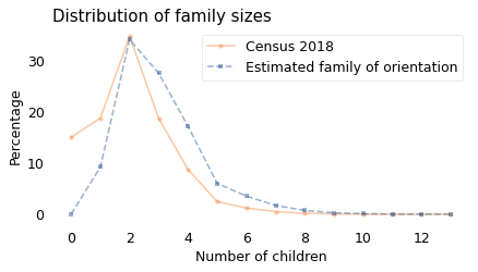
The circles show the percentage of women who bore each number of children. For example, about 15% of the women in the sample had no children; almost 35% of them had two.
Now, what would we see if we surveyed these children and asked them how many children their mothers had? Large families would be oversampled, small families would be undersampled, and families with no children would not appear at all. In general, a family with \(k\) children would appear in the sample \(k\) times.
So, if we take the distribution of family size from a sample of women, multiply each bar by the corresponding value of \(k\), and then divide through by the total, the result is the distribution of family size from a sample of children. In the previous figure, the square markers show this distribution.
As expected, children would report more large families (three or more children), fewer families with one child, and no families with zero children.
In general, the average family size is smaller if we survey women than if we survey their children. In this example, the average reported by women is close to 2; the average reported by their children would be close to 3.
So you might expect that, if family sizes reported by women get bigger, family sizes reported by children would get bigger, too. But that is not always the case, as we’ll see in the next section.
The Depression and the Baby Boom#
Preston used data from the U.S. Census Bureau to compare family sizes at several points between 1890 and 1970. Among the results, he finds:
In 1950, the average family size reported by the women in the survey was 2.3. In 1970, it was 2.7. This increase was not surprising because the first group did most of their childbearing during the Great Depression, the second group mostly during the Baby Boom.
However, if we survey the children of these women, and ask about their mothers, the average in the 1950 sample would be 4.9; in the 1970 sample it would be 4.5. This decrease was surprising.
According to the women in the survey, families got bigger between 1950 and 1970, by almost half a child. According to their children, families got smaller during the same interval, by almost half a child.
It doesn’t seem like both can be true, but they are. To understand why, we have to look at the whole distribution of family size, not just the averages.
Preston’s paper presents the distributions in a figure, so I used a graph digitizing tool to extract them numerically. Because this process introduces small errors, I adjusted the results to match the average family sizes Preston computed. The following figure shows these distributions.
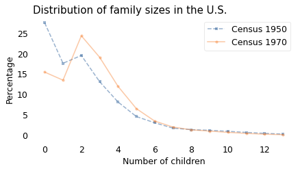
The biggest differences are in the left part of the curve. The women surveyed in 1950 were substantially more likely to have zero children or one, compared to women surveyed in 1970. They were less likely to have 2–5 children, and slightly more likely to have 9 or more.
Looking at it another way, family size was more variable in the 1950 cohort. The standard deviation of the distribution was about 2.4; in the 1970 cohort it was about 2.2. This variability is the reason for the difference between the two ways of measuring family size.
As Preston derived, there is a mathematical relationship between the average family size as reported by women, which he calls \(X\), and the average family size as reported by their children, which he calls \(C\).
\(C = X + V/X\)
where \(V\) is the variance of the distribution (the square of standard deviation).
Compared to 1950, \(X\) was bigger in 1970, but \(V\) was smaller; and as it turns out, \(C\) was smaller, too. That’s how family sizes can be bigger if we survey mothers and smaller if we survey their children.
More Recently#
With more recent Census data, we can see what has happened to family sizes since 1970.
The following figure shows the average number of children born to women aged 40-44 when they were surveyed. The first cohort was interviewed in 1976, the last in 2018.
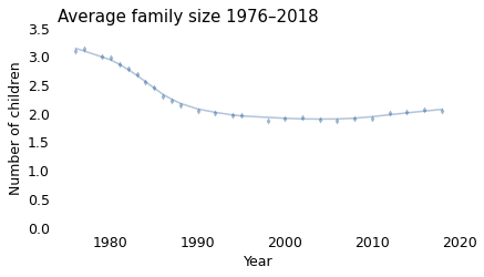
Between 1976 and 1990, average family size fell from more than 3 to less than 2. Since 2010, it has increased a little.
To see where those changes came from, let’s see how each part of the distribution has changed. The following figure shows the percentage of women with 0, 1, or 2 children, plotted over time.
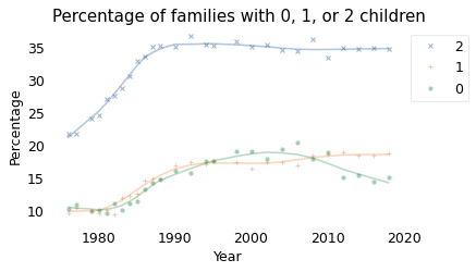
The fraction of small families has increased; most notably, between 1976 and 1990, the percentage of women with two children increased from 22% to 35%. The percentage of women with one child or zero also increased.
The following figure shows how the percentage of large families changed over the same period.
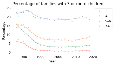
The proportion of large families declined substantially, especially the percentage of families with 5-6 children, which was 14% in 1976 and 4% in 2018. Over the same period, the percentage of families with seven or more children declined from 6% to less than 1%.
We can use this data to see how the two measures of family size have changed over time.
The following figure shows \(X\), which is the average number of children ever born to the women who were surveyed, and \(C\), which is the average we would measure if we surveyed their children.
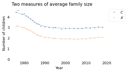
Between 1976 and 1990, the average family size reported by women, \(X\), decreased from 3.1 to 2.0. Over the same period, the average family size reported by children, \(C\), decreased from 4.4 to 2.8. Since 1990, \(X\) has been close to 2 and \(C\) has been close to 3.
Preston’s Paradox#
Now we are ready to explain the surprising result from the imaginary kingdom at the beginning of the chapter. In the scenario, the average family size was 3. Then we enacted a new law requiring every woman to have fewer children than her mother. In perfect compliance with the law, every woman had fewer children than her mother. Nevertheless, 25 years later the average family size was 3.3.
How is that possible?
As it happens, the numbers in the scenario are not contrived; they are based on the actual distribution of family size in the United States in 1979. Among the women who were interviewed that year, the average family size was close to 3.
Of course, nothing like the “fewer than mother” law was implemented in the U.S., and 25 years later the average family size was 1.9, not 3.3. But using the actual distribution as a starting place, we can simulate what would have happened in different scenarios.
First, let’s suppose that every woman has the same number of children as her mother. At first, you might think that the distribution of family size would not change, but that’s not right. In fact, family sizes would increase quickly.
As a small example, suppose there are only two families, one with two children and the other with four, so the average family size is three.
Assuming that half of the children are girls, in the next generation there would be one woman from a two-child family and two from a four-child family.
If each of these women has the same number of children as her mother, one would have two children and the other two would have four. So the average family size would be 3.33.
In the next generation, there would be one woman with two children, again, but there would be four with four. So the average family size would be 3.6.
In successive generations, the number of four-child families would increase exponentially, and the average family size would quickly approach to 4.
We can do the same calculation with a more realistic distribution. In fact, it is the same calculation we used to compute the distribution of family size as reported by children. In the same way large families are overrepresented when we survey children, large families are overrepresented in the next generation if every woman has the same number of children as her mother.
The following figure shows the actual distribution of family sizes from 1979 (solid line) and the result of this calculation, which simulates the “same as mother” scenario (dashed line).
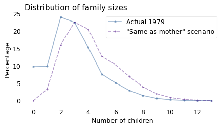
In the next generation, there are fewer small families and more big families, so the distribution is shifted to the right. The mean of the original distribution is 3; the mean of the simulated distribution is 4.3.
If we repeat the process, the average family size would be 5.2 in the next generation, 6.1 in the next, and 6.9 in the next. Eventually, nearly all women would have 13 children, which is the maximum in this dataset.
Observing this pattern, Preston explains:
The implications for population growth are obvious. Members of each generation must, on average, bear substantially fewer children than were born into their own family of orientation merely to keep population fertility rates constant.
So let’s see what happens if we follow Preston’s advice.
One Child Fewer#
Suppose every woman has precisely one child fewer than her mother. We can simulate this behavior by computing the biased distribution, as in the previous section, and then shifting the result one child to the left.
The following figure shows the actual distribution from 1979 again, along with the result of this simulation.
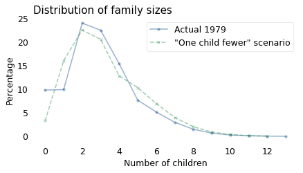
The simulated distribution has been length-biased, which increases the average, and then shifted to the left, which decreases the average. In general, the net effect could be an increase or a decrease; in this example, it’s an increase from 3.0 to 3.3.
In The Long Run#
If we repeat this process and simulate the next generation, the average family size increases again, to 3.5. In the next generation it increases to 3.8.
It might seem like it would increase forever, but if every woman has one child fewer than her mother, in each generation the maximum family size decreases by one. So eventually the average comes down.
The following figure shows the average family size over 10 generations, where Generation 0 follows the actual distribution from 1979.
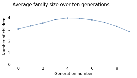
Family size would increase for four generations, peaking at 3.9. Then it would take another five generations to fall below the starting value. At 25 years per generation, that means it would take more than 200 years for the new law to have the desired effect.
In Reality#
Of course, no such law was in effect in the United States between 1979 and 1990. Nevertheless, the average family size fell from close to 3 to close to 2. That’s an enormous change in less than one generation. How is that even possible? We’ve seen that it is not enough if every woman has one child fewer than her mother; the actual difference must have been larger.
In fact, the difference was about 2.3. To see why, remember that the average family size, as seen by the children of the women surveyed in 1979, was 4.3. But when those children grew up and the women among them were surveyed in 1990, they reported an average family size close to 2. So on average, they had 2.3 fewer children than their mothers.
As Preston explains:
A major intergenerational change at the individual level is required in order to maintain intergenerational stability at the aggregate level.
Those who exhibit the most traditional behavior with respect to marriage and women’s roles will always be overrepresented as parents of the next generation, and a perpetual disaffiliation from their model by offspring is required in order to avert an increase in traditionalism for the population as a whole.
In other words, children have to reject the childbearing example of their mothers; otherwise, we are all doomed.
In the Present#
The women surveyed in 1990 rejected the childbearing example of their mothers emphatically. On average, each woman had 2.3 fewer children than her mother. If that pattern had continued for another generation, the average family size in 2018 would have been about 0.8. But it wasn’t.
In fact, the average family size in 2018 was very close to 2, just as in 1990. So how did that happen?
As it turns out, this is close to what we would expect if every woman had one child fewer than her mother. The following distribution shows the actual distribution in 2018, compared to the result if we start with the 1990 distribution and simulate the “one child fewer” scenario.
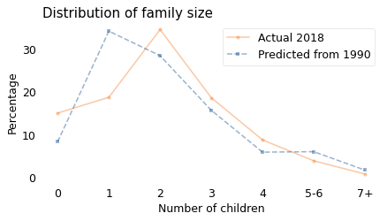
The means of the two distributions are almost the same, but the shapes are different. In reality, there were more zero- and two-child families in 1990 than the simulation predicts, and fewer one-child families. But at least on average, it seems like women in the U.S. have been following the “one child fewer” policy for the last 30 years.
The scenario at the beginning of this chapter is meant to be light-hearted, but in reality governments in many places and times have enacted policies meant to control family sizes and population growth. Most famously, China implemented a one-child policy in 1980 that imposed severe penalties on families with more than one child. Of course, this policy is objectionable to anyone who considers reproductive freedom a fundamental human right. But even as a practical matter, the unintended consequences were profound.
Rather than catalog them, I will mention one that is particularly ironic: while this policy was in effect, economic and social forces reduced the average desired family size so much that, when the policy was relaxed in 2015 and again in 2021, average lifetime fertility increased to only 1.3, far below the level needed to keep the population constant, near 2.1. Since then, China has implemented new policies intended to increase family sizes, but it is not clear whether they will have much effect. Demographers predict that by the time you read this, the population of China will probably be shrinking. The consequences of the one-child policy are widespread and will affect China and the rest of the world for a long time.